1. Getting started with Python

This open-access textbook is, and will remain, freely available for everyone’s enjoyment (also in PDF; a paper copy can also be ordered). It is a non-profit project. Although available online, it is a whole course, and should be read from the beginning to the end. Refer to the Preface for general introductory remarks. Any bug/typo reports/fixes are appreciated. Make sure to check out Deep R Programming [36] too.

1.1. Installing Python

Python was designed and implemented by the Dutch programmer Guido van Rossum in the late 1980s. It is an immensely popular object-orientated programming language. Over the years, it proved particularly suitable for rapid prototyping. Its name is a tribute to the funniest British comedy troupe ever. We will surely be having a jolly good laugh[1] along our journey.

In this course, we will be relying on the reference implementation of the Python language (called CPython[2]), version 3.11 (or any later one).

Users of UNIX-like operating systems (GNU/Linux[3], FreeBSD, etc.) may download Python via their native package manager (e.g., sudo apt install python3 in Debian and Ubuntu). Then, additional Python packages (see Section 1.4) can be installed by the said manager or directly from the Python Package Index (PyPI) via the pip tool.

Users of other operating systems can download Python from the project’s website or some other distribution available on the market, e.g., Anaconda or Miniconda.

Exercise 1.1

Install Python on your computer.

1.2. Working with Jupyter notebooks

Jupyter brings a web browser-based development environment supporting numerous programming languages. Even though, in the long run, it is not the most convenient space for exercising data science in Python (writing standalone scripts in some more advanced editors is the preferred option), we chose it here because of its educative advantages (interactivity, beginner-friendliness, etc.).

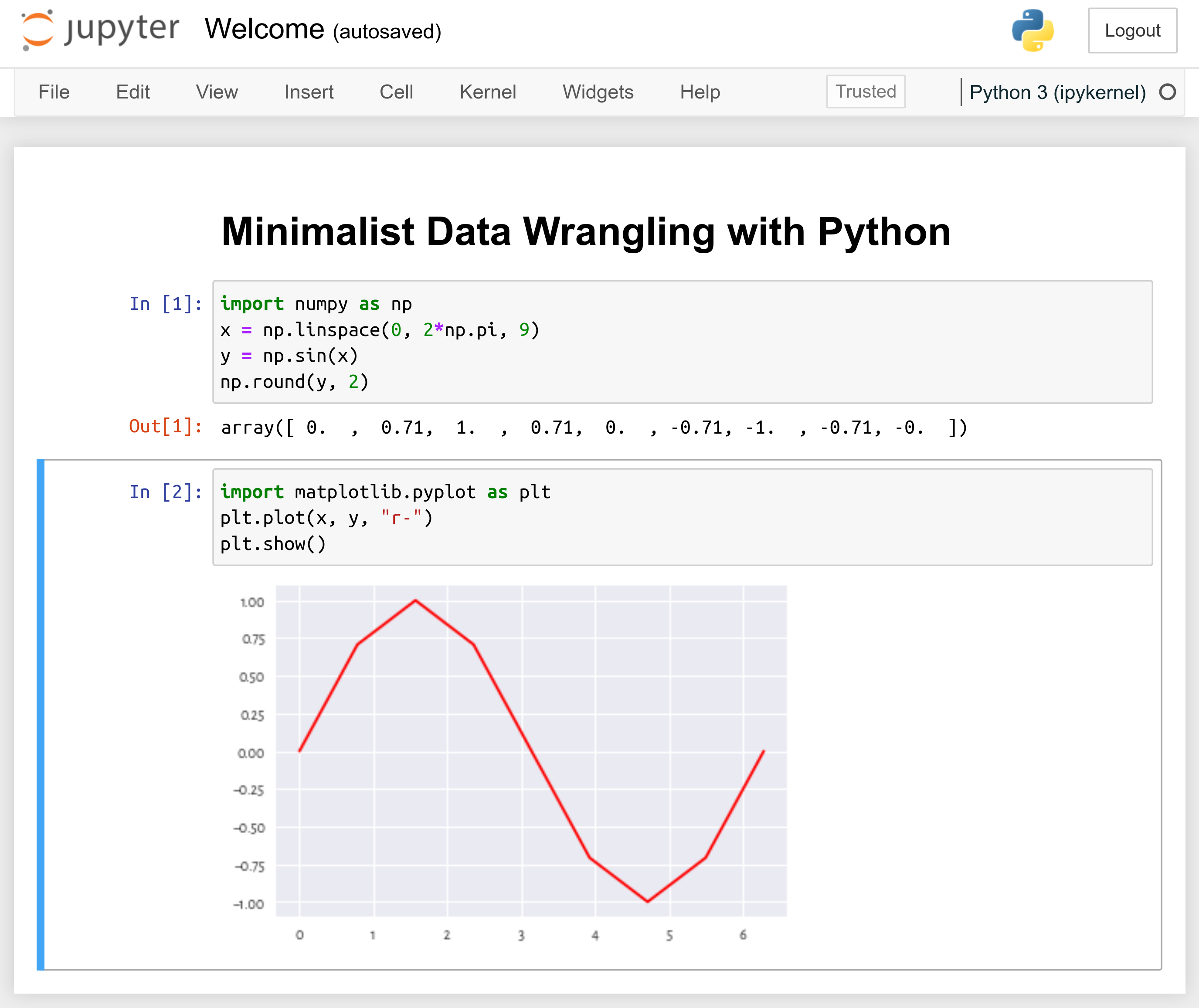
Figure 1.1 An example Jupyter notebook.

In Jupyter, we can work with:

• Jupyter notebooks — .ipynb documents combining code, text, plots, tables, and other rich outputs; importantly, code chunks can be created, modified, and run, which makes it a fine reporting tool for our common data science needs; see Figure 1.1;

• code consoles — terminals where we evaluate code chunks in an interactive manner (a read-eval-print loop);

• source files in a variety of programming languages — with syntax highlighting and the ability to send code to the associated consoles;

and many more.

Exercise 1.2

Head to the official documentation of the Jupyter project. Watch the introductory video linked in the Get Started section.

Note

(*) More advanced students might consider, for example, jupytext as a means to create .ipynb files directly from Markdown documents.

1.2.1. Launching JupyterLab

How we launch JupyterLab (or its lightweight version, Jupyter Notebook) will vary from system to system. We all need to determine the best way to do it by ourselves.

Some users will be able to start JupyterLab via their start menu/application launcher. Alternatively, we can open the system terminal (bash, zsh, etc.) and type:

cd our/favourite/directory  # change directory
jupyter lab  # or jupyter-lab, depending on the system

This should launch the JupyterLab server and open the corresponding app in our favourite web browser.

Note

Some commercial cloud-hosted instances or forks of the open-source JupyterLab project are available on the market, but we endorse none of them; even though they might be provided gratis, there are always strings attached. It is best to run our applications locally, where we are free to be in full control over the software environment. Contrary to the former solution, we do not have to remain on-line to use it.

1.2.2. First notebook

Follow the undermentioned steps to create your first notebook.

1. From JupyterLab, create a new notebook running a Python 3 kernel, for example, by selecting File \(\to\) New \(\to\) Notebook from the application menu.

2. Select File \(\to\) Rename Notebook and change the filename to HelloWorld.ipynb.

   Important

   The file is stored relative to the running JupyterLab server instance’s current working directory. Make sure you can locate HelloWorld.ipynb on your disk using your file explorer. On a side note, .ipynb is just a JSON file that can also be edited using ordinary text editors.

3. In the first code cell, input:

   print("G'day!")
   

4. Press Ctrl+Enter (or Cmd+Return on m**OS) to execute the code cell and display the result; see Figure 1.2.

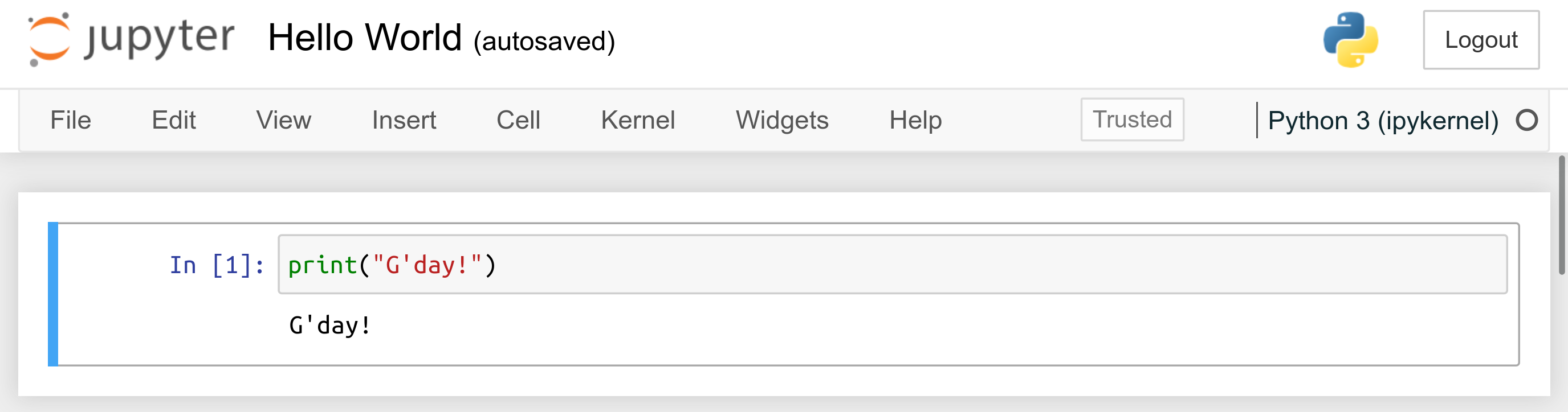
Figure 1.2 “Hello, World” in a Jupyter notebook.

1.2.3. More cells

We are on fire. We cannot stop now.

1. By pressing Enter, we enter the Edit mode. Modify the current cell’s contents so that it becomes:

   # My first code cell (this is a comment)
   print("G'day!")  # prints a message (this is a comment too)
   print(2+5)  # prints a number
   

2. Press Ctrl+Enter to execute whole code chunk and replace the previous outputs with the updated ones.

3. Enter another command that prints a message that you would like to share with the world. Note that character strings in Python must be enclosed either in double quotes or in apostrophes.

4. Press Shift+Enter to execute the current code cell, create a new one below it, and then enter the edit mode.

5. In the new cell, input and then execute:

   import matplotlib.pyplot as plt  # the main plotting library
   plt.bar(
       ["Python", "JavaScript", "HTML", "CSS"],  # a list of strings
       [80, 30, 10, 15]  # a list of integers (the respective bar heights)
   )
   plt.title("What makes you happy?")
   plt.show()
   

6. Add three more code cells that display some text or create other bar plots.

Exercise 1.3

Change print(2+5) to PRINT(2+5). Run the corresponding code cell and see what happens.

Note

In the Edit mode, JupyterLab behaves like an ordinary text editor. Most keyboard shortcuts known from elsewhere are available, for example:

• Shift+LeftArrow, DownArrow, UpArrow, or RightArrow – select text,

• Ctrl+c – copy,

• Ctrl+x – cut,

• Ctrl+v – paste,

• Ctrl+z – undo,

• Ctrl+] – indent,

• Ctrl+[ – dedent,

• Ctrl+/ – toggle comment.

1.2.4. Edit vs command mode

By pressing ESC, we can enter the Command mode.

1. Use the arrow DownArrow and UpArrow keys to move between the code cells.

2. Press d,d (d followed by another d) to delete the currently selected cell.

3. Press z to undo the last operation.

4. Press a and b to insert a new blank cell, respectively, above and below the current one.

5. Note a simple drag and drop can relocate cells.

Important

ESC and Enter switch between the Command and Edit modes, respectively.

Example 1.4

In Jupyter notebooks, the linear flow of chunks’ execution is not strongly enforced. For instance:

## In  [2]:
            x = [1, 2, 3]

## In  [10]:
            sum(x)
## Out [10]:
##          18

## In  [7]:
            sum(y)
## Out [7]:
##          6

## In  [6]:
            x = [5, 6, 7]

## In  [5]:
            y = x

The chunk IDs reveal the true order in which the author has executed them. By editing cells in a rather frivolous fashion, we may end up with matter that makes little sense when it is read from the beginning to the end. It is thus best to always select Restart Kernel and Run All Cells from the Kernel menu to ensure that evaluating content step by step renders results that meet our expectations.

1.2.5. Markdown cells

So far, we have only been playing with code cells. Notebooks are not just about writing code, though. They are meant to be read by humans too. Thus, we need some means to create formatted text.

Markdown is lightweight yet powerful enough markup (pun indented) language widely used on many popular platforms (e.g., on Stack Overflow and GitHub). We can convert the current cell to a Markdown block by pressing m in the Command mode (note that by pressing y we can turn it back to a code cell).

1. In a new Markdown cell, enter:

   # Section
   
   ## Subsection
   
   This is the first paragraph. It ~~was~~ *is* **very** nice.
   Great success.
   
   This is the second paragraph. Note that a blank line separates
   it from the previous one. And now for something completely different:
   a bullet list:
   
   * one
   
   * two
   
       1. aaa
   
       2. bbbb
   
   * [three](https://en.wikipedia.org/wiki/3)
   
   
   ```python
   # some code to display (but not execute)
   2+2
   ```
   
   ![Python logo](https://www.python.org/static/img/python-logo.png)
   

2. Press Ctrl+Enter to display the formatted text.

3. Notice that Markdown cells can be modified in the Edit mode as usual (the Enter key).

Exercise 1.5

Read the official introduction to the Markdown syntax.

Exercise 1.6

Follow this interactive Markdown tutorial.

Exercise 1.7

Apply what you have learnt by making the current Jupyter notebook more readable. At the beginning of the report, add a header featuring your name and email address. Before and after each code cell, explain its purpose and how to interpret the obtained results.

1.3. The best note-taking app

Our learning will not be effective if we do note take good note of the concepts that we come across during this course, especially if they are new to us. More often than not, we will find ourselves in a need to write down the definitions and crucial properties of the methods we discuss, draw simple diagrams and mind maps to build connections between different topics, verify the validity of some results, or derive simple mathematical formulae ourselves.

Let’s not waste our time finding the best app for our computers, phones, or tablets. One versatile note-taking solution is an ordinary piece of A4 paper and a pen or a pencil. Loose sheets, 5 mm grid-ruled for graphs and diagrams, work nicely. They can be held together using a cheap landscape clip folder (the one with a clip on the long side). This way, it can be browsed through like an ordinary notebook. Also, new pages can be added anywhere, and their ordering altered arbitrarily.

1.4. Initialising each session and getting example data

From now on, we assume that the following commands are issued at the beginning of each Python session.

# import key packages (required):
import numpy as np
import scipy.stats
import pandas as pd
import matplotlib.pyplot as plt
import seaborn as sns


# further settings (optional):
pd.set_option("display.notebook_repr_html", False)  # disable "rich" output

import os
os.environ["COLUMNS"] = "74"  # output width, in characters
np.set_printoptions(
    linewidth=74,   # output width
    legacy="1.25",  # print scalars without type information
)
pd.set_option("display.width", 74)

import sklearn
sklearn.set_config(display="text")

plt.style.use("seaborn-v0_8")  # plot style template

_colours = [  # the "R4" palette from R
    "#000000f0", "#DF536Bf0", "#61D04Ff0", "#2297E6f0",
    "#28E2E5f0", "#CD0BBCf0", "#F5C710f0", "#999999f0"
]

_linestyles = [
    "solid", "dashed", "dashdot", "dotted"
]

plt.rcParams["axes.prop_cycle"] = plt.cycler(
    # each plotted line will have a different plotting style
    color=_colours, linestyle=_linestyles*2
)
plt.rcParams["patch.facecolor"] = _colours[0]

np.random.seed(123)  # initialise the pseudorandom number generator

First, we imported the most frequently used packages (together with their usual aliases, we will get to that later). Then, we set up some further options that yours truly is particularly fond of. On a side note, Section 6.4.2 discusses the issues in reproducible pseudorandom number generation.

Open-source software regularly enjoys feature extensions, API changes, and bug fixes. It is worthwhile to know which version of the Python environment was used to execute all the code listed in this book:

import sys
print(sys.version)
## 3.11.10 (main, Sep 09 2024, 17:03:08) [GCC]

Given beneath are the versions of the packages that we will be relying on. This information can usually be accessed by calling print(package.__version__).

Package	Version
numpy	2.1.1
scipy	1.14.1
matplotlib	3.9.0
pandas	2.2.2
seaborn	0.13.2
sklearn (scikit-learn) (*)	1.5.1
icu (PyICU) (*)	2.13.1
IPython (*)	8.27.0
mplfinance (*)	0.12.10b0

We expect 99% of our code to work in the (near-)future versions of the environment. If the diligent reader discovers that this is not the case, for the benefit of other students, filing a bug report at https://github.com/gagolews/datawranglingpy will be much appreciated.

Important

All example datasets that we use throughout this course are available for download at https://github.com/gagolews/teaching-data.

Exercise 1.8

Ensure you know hot to access the files from our teaching data repository. Chose any file, e.g., nhanes_adult_female_height_2020.txt in the marek folder, and then click Raw. It is the URL where you have been redirected to, not the previous one, that includes the link to be used from within your Python session. Also, note that each dataset starts with several comment lines explaining its structure, the meaning of the variables, etc.

1.5. Exercises

Exercise 1.9

What is the difference between the Edit and the Command mode in Jupyter?

Exercise 1.10

How can we format a table in Markdown? How can we insert an image, a hyperlink, and an enumerated list?

---

[1]

When we are all in tears because of mathematics and programming, those that we shed are often tears of joy.

[2]

(*) CPython was written in the C programming language. Many Python packages are just convenient wrappers around code written in C, C++, or Fortran.

[3]

GNU/Linux is the operating system of choice for machine learning engineers and data scientists both on the desktop and in the cloud. Switching to a free system at some point cannot be recommended highly enough.