15. Missing, censored, and questionable data

This open-access textbook is, and will remain, freely available for everyone’s enjoyment (also in PDF; a paper copy can also be ordered). It is a non-profit project. Although available online, it is a whole course, and should be read from the beginning to the end. Refer to the Preface for general introductory remarks. Any bug/typo reports/fixes are appreciated. Make sure to check out Deep R Programming [36] too.

Up to now, we have been mostly assuming that observations are of decent quality, i.e., trustworthy. It would be nice if that was always the case, but it is not.

In this chapter, we briefly address the most rudimentary methods for dealing with suspicious observations: outliers, missing, censored, imprecise, and incorrect data.

15.1. Missing data

Consider an excerpt from National Health and Nutrition Examination Survey that we played with in Chapter 12:

nhanes = pd.read_csv("https://raw.githubusercontent.com/gagolews/" +
    "teaching-data/master/marek/nhanes_p_demo_bmx_2020.csv",
    comment="#")
nhanes.loc[:, ["BMXWT", "BMXHT", "RIDAGEYR", "BMIHEAD", "BMXHEAD"]].head()
##    BMXWT  BMXHT  RIDAGEYR  BMIHEAD  BMXHEAD
## 0    NaN    NaN         2      NaN      NaN
## 1   42.2  154.7        13      NaN      NaN
## 2   12.0   89.3         2      NaN      NaN
## 3   97.1  160.2        29      NaN      NaN
## 4   13.6    NaN         2      NaN      NaN

Some of the columns bear NaN (not-a-number) values. They are used here to encode missing (not available) data. Previously, we decided not to be bothered by them: a shy call to dropna resulted in their removal. But we are curious now.

The reasons behind why some items are missing might be numerous, in particular:

• a participant did not know the answer to a given question;

• someone refused to answer a given question;

• a person did not take part in the study anymore (attrition, death, etc.);

• an item was not applicable (e.g., number of minutes spent cycling weekly when someone answered they did not learn to ride a bike yet);

• a piece of information was not collected, e.g., due to the lack of funding or a failure of a piece of equipment.

15.1.1. Representing and detecting missing values

Sometimes missing values are specially encoded, especially in CSV files, e.g., with -1, 0, 9999, numpy.inf, -numpy.inf, or None, strings such as "NA", "N/A", "Not Applicable", "---". This is why we must always inspect our datasets carefully. To assure consistent representation, we can convert them to NaN (as in: numpy.nan) in numeric (floating-point) columns or to Python’s None otherwise.

Vectorised functions such as numpy.isnan (or, more generally, numpy.isfinite) and pandas.isnull as well as isna methods for the DataFrame and Series classes verify whether an item is missing or not.

For instance, here are the counts and proportions of missing values in selected columns of nhanes:

nhanes.isna().apply([np.sum, np.mean]).T.nlargest(5, "sum")  # top 5 only
##               sum      mean
## BMIHEAD   14300.0  1.000000
## BMIRECUM  14257.0  0.996993
## BMIHT     14129.0  0.988042
## BMXHEAD   13990.0  0.978322
## BMIHIP    13924.0  0.973706

Looking at the column descriptions on the data provider’s website, for example, BMIHEAD stands for “Head Circumference Comment”, whereas BMXHEAD is “Head Circumference (cm)”, but these were only collected for infants.

Exercise 15.1

Read the column descriptions (refer to the comments in the CSV file for the relevant URLs) to identify the possible reasons for some of the records in nhanes being missing.

Exercise 15.2

Learn about the difference between the pandas.DataFrameGroupBy.size and pandas.DataFrameGroupBy.count methods.

15.1.2. Computing with missing values

Our using NaN to denote a missing piece of information is merely an ugly (but functional) hack[1]. The original use case for not-a-number is to represent the results of incorrect operations, e.g., logarithms of negative numbers or subtracting two infinite entities. We thus need extra care when handling them.

Generally, arithmetic operations on missing values yield a result that is undefined as well:

np.nan + 2  # "don't know" + 2 == "don't know"
## nan
np.mean([1, np.nan, 2, 3])
## nan

There are versions of certain aggregation functions that ignore missing values whatsoever: numpy.nanmean, numpy.nanmin, numpy.nanmax, numpy.nanpercentile, numpy.nanstd, etc.

np.nanmean([1, np.nan, 2, 3])
## 2.0

Regrettably, running these aggregation functions directly on Series objects ignores missing entities by default. Compare an application of numpy.mean on a Series instance vs on a vector:

x = nhanes.head().loc[:, "BMXHT"]  # some example Series, whatever
np.mean(x), np.mean(np.array(x))
## (134.73333333333332, nan)

This is unfortunate a behaviour as this way we might miss (sic!) the presence of missing values. Therefore, it is crucial to have the dataset carefully inspected in advance.

Also, NaN is of the floating-point type. As a consequence, it cannot be present in, amongst others, logical vectors.

x  # preview
## 0      NaN
## 1    154.7
## 2     89.3
## 3    160.2
## 4      NaN
## Name: BMXHT, dtype: float64
y = (x > 100)
y
## 0    False
## 1     True
## 2    False
## 3     True
## 4    False
## Name: BMXHT, dtype: bool

Unfortunately, comparisons against missing values yield False, instead of the more semantically valid missing value. Hence, if we want to retain the missingness information (we do not know if a missing value is greater than 100), we need to do it manually:

y = y.astype("object")  # required for numpy vectors, not for pandas Series
y[np.isnan(x)] = None
y
## 0     None
## 1     True
## 2    False
## 3     True
## 4     None
## Name: BMXHT, dtype: object

Exercise 15.3

Read the pandas documentation about missing value handling.

15.1.3. Missing at random or not?

At a general level (from the mathematical modelling perspective), we may distinguish between a few missingness patterns [83]:

• missing completely at random: reasons are unrelated to data and probabilities of cases’ being missing are all the same;

• missing at random: there are different probabilities of being missing within distinct groups (e.g., ethical data scientists might tend to refuse to answer specific questions);

• missing not at random: due to reasons unknown to us (e.g., data was collected at different times, there might be significant differences within the groups that we cannot easily identify, e.g., amongst participants with a background in mathematics where we did not ask about education or occupation).

It is important to try to determine the reason for missingness. This will usually imply the kinds of techniques that are suitable in specific cases.

15.1.4. Discarding missing values

We may try removing (discarding) rows or columns that carry at least one, some, or too many missing values. Nonetheless, such a scheme will obviously not work for small datasets, where each observation is precious[2].

Also, we ought not to exercise data removal in situations where missingness is conditional (e.g., data only available for infants) or otherwise group-dependent (not completely at random). Otherwise, for example, it might result in an imbalanced dataset.

Exercise 15.4

With the nhanes_p_demo_bmx_2020 dataset, perform what follows.

1. Remove all columns that are comprised of missing values only.

2. Remove all columns that are made of more than 20% missing values.

3. Remove all rows that only consist of missing values.

4. Remove all rows that bear at least one missing value.

5. Remove all columns that carry at least one missing value.

Hint: pandas.DataFrame.dropna might be useful in the simplest cases, and numpy.isnan or pandas.DataFrame.isna with loc[...] or iloc[...] can be applied otherwise.

15.1.5. Mean imputation

When we cannot afford or it is inappropriate/inconvenient to proceed with the removal of missing observations or columns, we may try applying some missing value imputation techniques. Let’s be clear, though: this is merely a replacement thereof by some hopefully adequate guesstimates.

Important

In all kinds of reports from data analysis, we need to be explicit about the way we handle the missing values. Sometimes they might strongly affect the results.

Consider an example vector with missing values, comprised of heights of the adult participants of the NHANES study.

x = nhanes.loc[nhanes.loc[:, "RIDAGEYR"] >= 18, "BMXHT"]

The simplest approach is to replace each missing value with the corresponding column’s mean. This does not change the overall average but decreases the variance.

xi = x.copy()
xi[np.isnan(xi)] = np.nanmean(xi)

Similarly, we could consider replacing missing values with the median, or – in the case of categorical data – the mode.

Furthermore, we expect heights to differ, on average, between sexes. Consequently, another imputation option is to replace the missing values with the corresponding within-group averages:

xg = x.copy()
g = nhanes.loc[nhanes.loc[:, "RIDAGEYR"] >= 18, "RIAGENDR"]
xg[np.isnan(xg) & (g == 1)] = np.nanmean(xg[g == 1])  # male
xg[np.isnan(xg) & (g == 2)] = np.nanmean(xg[g == 2])  # female

Unfortunately, whichever imputation method we choose, will artificially distort the data distribution and introduce some kind of bias; see Figure 15.1 for the histograms of x, xi, and xg. These effects can be obscured if we increase the histogram bins’ widths, but they will still be present in the data. No surprise here: we added to the sample many identical values.

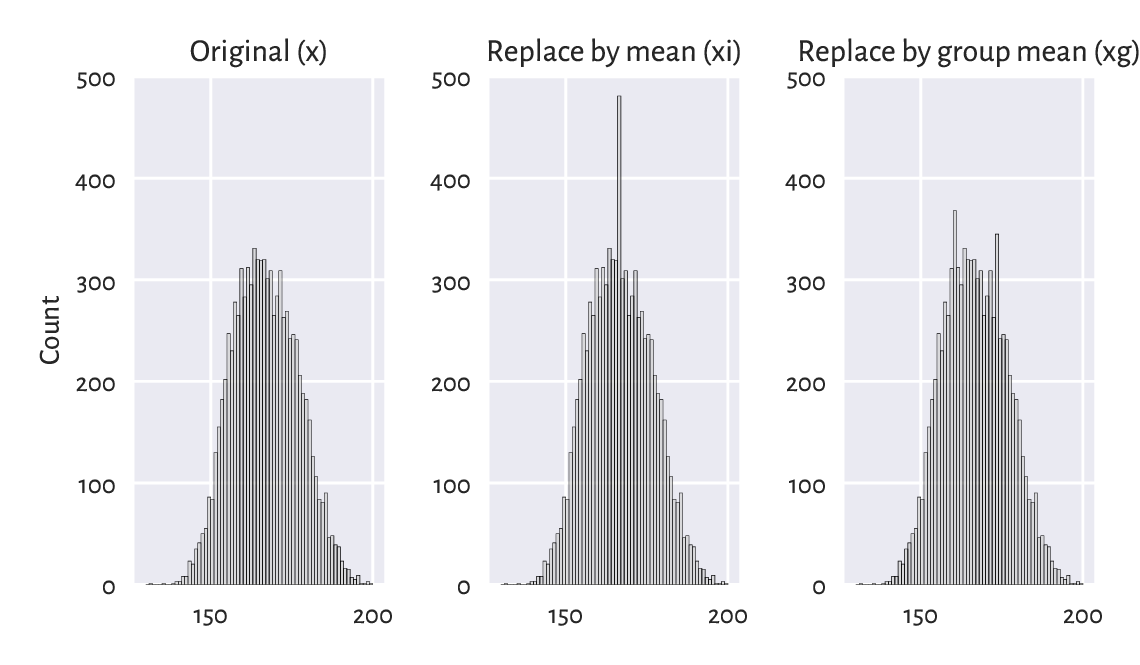
Figure 15.1 The mean imputation distorts the data distribution.

Exercise 15.5

With the nhanes_p_demo_bmx_2020 dataset, perform what follows.

1. For each numerical column, replace all missing values with the column averages.

2. For each categorical column, replace all missing values with the column modes.

3. For each numerical column, replace all missing values with the averages corresponding to a patient’s sex (as given by the RIAGENDR column).

15.1.6. Imputation by classification and regression (*)

We can easily compose a missing value imputer based on averaging data from an observation’s non-missing nearest neighbours; compare Section 9.2.1 and Section 12.3.1. This is an extension of the simple idea of finding the most similar observation (with respect to chosen criteria) to a given one and then borrowing non-missing measurements from it.

More generally, different regression or classification models can be built on non-missing data (training sample) and then the missing observations can be replaced by the values predicted by those models.

Note

(**) Rubin (e.g., in [62]) suggests the use of a procedure called multiple imputation (see also [92]), where copies of the original datasets are created, missing values are imputed by sampling from some estimated distributions, the inference is made, and then the results are aggregated. An example implementation of such an algorithm is available in sklearn.impute.IterativeImputer.

15.2. Censored and interval data (*)

Censored data frequently appear in the context of reliability, risk analysis, and biostatistics, where the observed objects might fail (e.g., break down, die, withdraw; compare, e.g., [66]). Our introductory course cannot obviously cover everything. However, a beginner analyst needs to be at least aware of the existence of:

• right-censored data: we only know that the actual value is greater than the recorded one (e.g., we stopped the experiment on the reliability of light bulbs after 1000 hours, so those which still work will not have their time-of-failure precisely known);

• left-censored data: the true observation is less than the recorded one, e.g., we observe a component’s failure, but we do not know for how long it has been in operation before the study has started.

In such cases, the recorded datum of, say, 1000, can essentially mean \([1000, \infty)\), \([0, 1000]\), or \((-\infty, 1000]\).

There might also be instances where we know that a value is in some interval \([a, b]\). There are numerical libraries that deal with interval computations, and some data analysis methods exist for dealing with such a scenario.

15.3. Incorrect data

Missing data can already be marked in a given sample. But we also might be willing to mark some existing values as missing, e.g., when they are incorrect. For example:

• for text data, misspelled words;

• for spatial data, GPS coordinates of places out of this world, nonexistent zip codes, or invalid addresses;

• for date-time data, misformatted date-time strings, incorrect dates such as “29 February 2011”, an event’s start date being after the end date;

• for physical measurements, observations that do not meet specific constraints, e.g., negative ages, or heights of people over 300 centimetres;

• IDs of entities that simply do not exist (e.g., unregistered or deleted clients’ accounts);

and so forth.

To be able to identify and handle incorrect data, we need specific knowledge of a particular domain. Optimally, data validation techniques should already be employed on the data collection stage. For instance, when a user submits an online form.

There can be many tools that can assist us with identifying erroneous observations, e.g., spell checkers such as hunspell.

For smaller datasets, observations can also be inspected manually. In other cases, we might have to develop custom algorithms for detecting such bugs in data.

Exercise 15.6

Given some data frame with numeric columns only, perform what follows.

1. Check if all numeric values in each column are between 0 and 1000.

2. Check if all values in each column are unique.

3. Verify that all the rowwise sums add up to 1.0 (up to a small numeric error).

4. Check if the data frame consists of 0s and 1s only. Provided that this is the case, verify that for each row, if there is a 1 in some column, then all the columns to the right are filled with 1s too.

Many data validation methods can be reduced to operations on strings; see Chapter 14. They may be as simple as writing a single regular expression or checking if a label is in a dictionary of possible values but also as difficult as writing your own parser for a custom context-sensitive grammar.

Exercise 15.7

Once we import the data fetched from dirty sources, relevant information will have to be extracted from raw text, e.g., strings like "1" should be converted to floating-point numbers. In the sequel, we suggest several tasks that can aid in developing data validation skills involving some operations on text.

Given an example data frame with text columns (manually invented, please be creative), perform what follows.

1. Remove trailing and leading whitespaces from each string.

2. Check if all strings can be interpreted as numbers, e.g., "23.43".

3. Verify if a date string in the YYYY-MM-DD format is correct.

4. Determine if a date-time string in the YYYY-MM-DD hh:mm:ss format is correct.

5. Check if all strings are of the form (+NN) NNN-NNN-NNN or (+NN) NNNN-NNN-NNN, where N denotes any digit (valid telephone numbers).

6. Inspect whether all strings are valid country names.

7. (*) Given a person’s date of birth, sex, and Polish ID number PESEL, check if that ID is correct.

8. (*) Determine if a string represents a correct International Bank Account Number (IBAN) (note that IBANs have two check digits).

9. (*) Transliterate text to ASCII, e.g., "żółty ©" to "zolty (C)".

10. (**) Using an external spell checker, determine if every string is a valid English word.

11. (**) Using an external spell checker, ascertain that every string is a valid English noun in the singular form.

12. (**) Resolve all abbreviations by means of a custom dictionary, e.g., "Kat." → "Katherine", "Gr." → "Grzegorz".

15.4. Outliers

Another group of inspectionworthy observations consists of outliers. We can define them as the samples that reside in the areas of substantially lower density than their neighbours.

Outliers might be present due to an error, or their being otherwise anomalous, but they may also simply be interesting, original, or novel. After all, statistics does not give any meaning to data items; humans do.

What we do with outliers is a separate decision. We can get rid of them, correct them, replace them with a missing value (and then possibly impute), or analyse them separately. In particular, there is a separate subfield in statistics called extreme value theory that is interested in predicting the distribution of very large observations (e.g., for modelling floods, extreme rainfall, or temperatures); see, e.g., [6]. But this is a topic for a more advanced course; see, e.g., [52]. By then, let’s stick with some simpler settings.

15.4.1. The 3/2 IQR rule for normally-distributed data

For unidimensional data (or individual columns in matrices and data frames), the first few smallest and largest observations should usually be inspected manually. For instance, it might happen that someone accidentally entered a patient’s height in metres instead of centimetres: such cases are easily detectable. A data scientist is like a detective.

Let’s recall the rule of thumb discussed in the section on box-and-whisker plots (Section 5.1.4). For data that are expected to come from a normal distribution, everything that does not fall into the interval \([Q_1-1.5\mathrm{IQR}, Q_3+1.5\mathrm{IQR}]\) can be considered suspicious. This definition is based on quartiles only, so it is not affected by potential outliers (they are robust aggregates; compare [52]). Plus, the magic constant 1.5 is nicely round and thus easy to memorise (an attractive feature). It is not too small and not too large; for the normal distribution \(\mathrm{N}(\mu, \sigma)\), the aforementioned interval corresponds to roughly \([\mu-2.698\sigma, \mu+2.698\sigma]\), and the probability of obtaining a value outside of it is c. 0.7%. In other words, for a sample of size 1000 that is truly normally distributed (not contaminated by anything), only seven observations will be flagged. It is not a problem to inspect them by hand.

Note

(*) We can choose a different threshold. For instance, for the normal distribution \(\mathrm{N}(10, 1)\), even though the probability of observing a value greater than 15 is theoretically non-zero, it is smaller 0.000029%, so it is sensible to treat this observation as suspicious. On the other hand, we do not want to mark too many observations as outliers: inspecting them manually might be too labour-intense.

Exercise 15.8

For each column in nhanes_p_demo_bmx_2020, inspect a few smallest and largest observations and see if they make sense.

Exercise 15.9

Perform the foregoing separately for data in each group as defined by the RIAGENDR column.

15.4.2. Unidimensional density estimation (*)

For skewed distributions such as the ones representing incomes, there might be nothing wrong, at least statistically speaking, with very large isolated observations.

For well-separated multimodal distributions on the real line, outliers may sometimes also fall in between the areas of high density.

Example 15.10

That neither box plots themselves, nor the \(1.5\mathrm{IQR}\) rule might not be ideal tools for multimodal data is exemplified in Figure 15.2. Here, we have a mixture of \(\mathrm{N}(10, 1)\) and \(\mathrm{N}(25, 1)\) samples and four potential outliers at \(0\), \(15\), \(45\), and \(50\).

x = np.genfromtxt("https://raw.githubusercontent.com/gagolews/" +
    "teaching-data/master/marek/blobs2.txt")
plt.subplot(1, 2, 1)
plt.boxplot(x, vert=False)
plt.yticks([])
plt.subplot(1, 2, 2)
plt.hist(x, bins=50, color="lightgray", edgecolor="black")
plt.ylabel("Count")

plt.show()

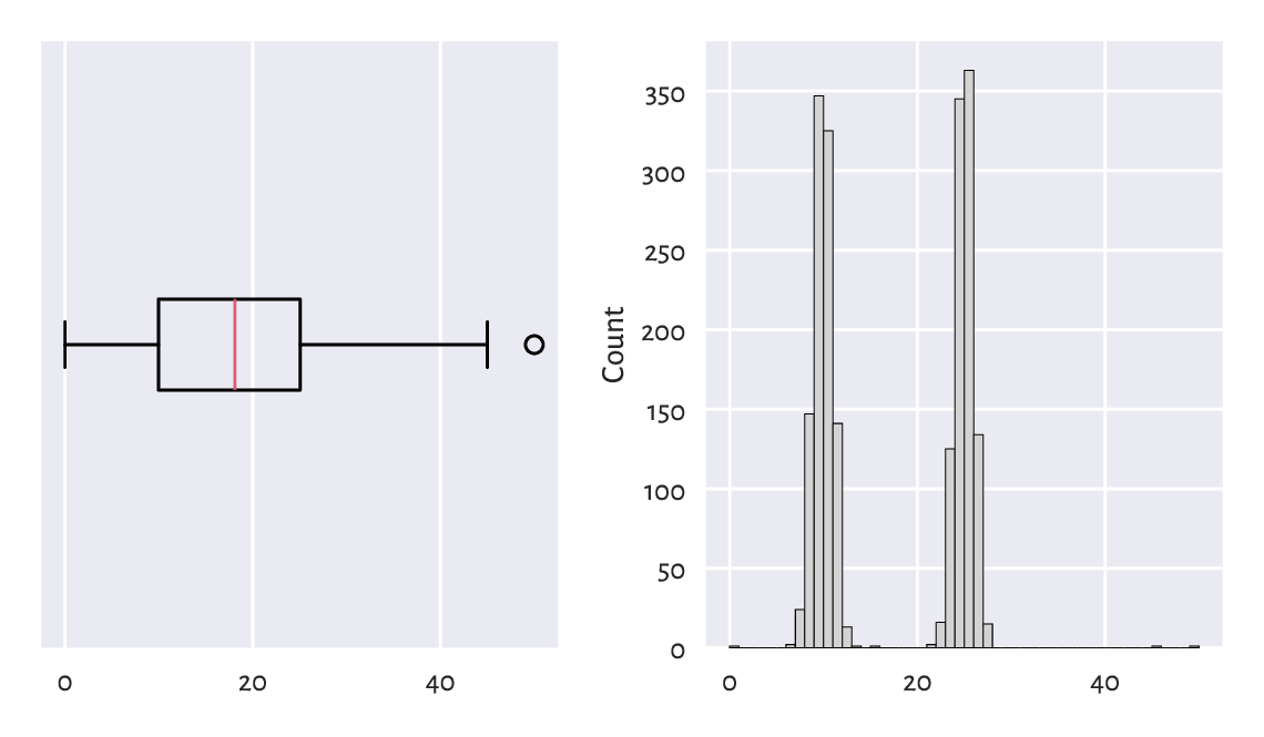
Figure 15.2 With box plots, we may fail to detect some outliers.

Fixed-radius search techniques discussed in Section 8.4 can be used for estimating the underlying probability density function. Given a data sample \(\boldsymbol{x}=(x_1,\dots,x_n)\), consider[3]:

\[ \hat{f}_r(z) = \frac{1}{2 r n} \sum_{i=1}^n |B_r(z)|, \]

where \(|B_r(z)|\) denotes the number of observations from \(\boldsymbol{x}\) whose distance to \(z\) is not greater than \(r\), i.e., fall into the interval \([z-r, z+r]\).

n = len(x)
r = 1  # radius – feel free to play with different values
import scipy.spatial
t = scipy.spatial.KDTree(x.reshape(-1, 1))
dx = pd.Series(t.query_ball_point(x.reshape(-1, 1), r)).str.len() / (2*r*n)
dx[:6]  # preview
## 0    0.000250
## 1    0.116267
## 2    0.116766
## 3    0.166667
## 4    0.076098
## 5    0.156188
## dtype: float64

Then, points in the sample lying in low-density regions (i.e., all \(x_i\) such that \(\hat{f}_r(x_i)\) is small) can be flagged for further inspection:

x[dx < 0.001]
## array([ 0.        , 13.57157922, 15.        , 45.        , 50.        ])

See Figure 15.3 for an illustration of \(\hat{f}_r\). Of course, \(r\) must be chosen with care, just like the number of bins in a histogram.

z = np.linspace(np.min(x)-5, np.max(x)+5, 1001)
dz = pd.Series(t.query_ball_point(z.reshape(-1, 1), r)).str.len() / (2*r*n)
plt.plot(z, dz, label=f"density estimator ($r={r}$)")
plt.hist(x, bins=50, color="lightgray", edgecolor="black", density=True)
plt.ylabel("Density")
plt.show()

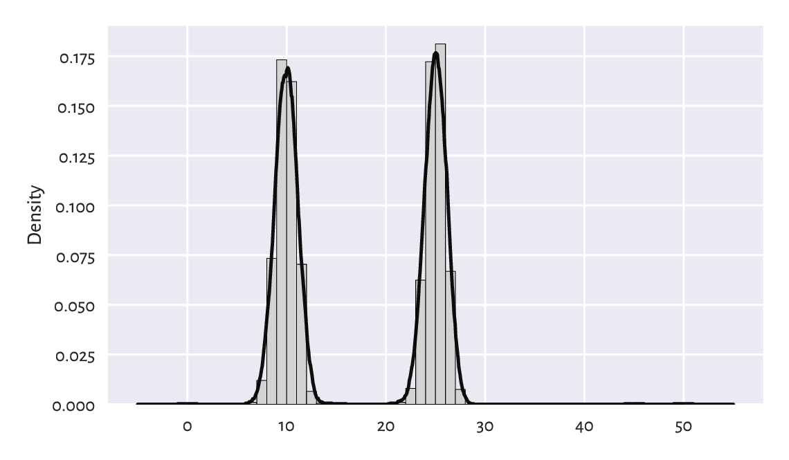
Figure 15.3 Density estimation based on fixed-radius search.

15.4.3. Multidimensional density estimation (*)

By far we should have become used to the fact that unidimensional data projections might lead to our losing too much information. Some values can seem perfectly fine when they are considered in isolation, but already plotting them in 2D reveals that the reality is more complex than that.

Figure 15.4 depicts the distributions of two natural projections of an example dataset:

X = np.genfromtxt("https://raw.githubusercontent.com/gagolews/" +
    "teaching-data/master/marek/blobs1.txt", delimiter=",")
plt.figure(figsize=(plt.rcParams["figure.figsize"][0], )*2)  # width=height
plt.subplot(2, 2, 1)
plt.boxplot(X[:, 0], vert=False)
plt.yticks([1], ["X[:, 0]"])
plt.subplot(2, 2, 2)
plt.hist(X[:, 0], bins=20, color="lightgray", edgecolor="black")
plt.title("X[:, 0]")
plt.subplot(2, 2, 3)
plt.boxplot(X[:, 1], vert=False)
plt.yticks([1], ["X[:, 1]"])
plt.subplot(2, 2, 4)
plt.hist(X[:, 1], bins=20, color="lightgray", edgecolor="black")
plt.title("X[:, 1]")
plt.show()

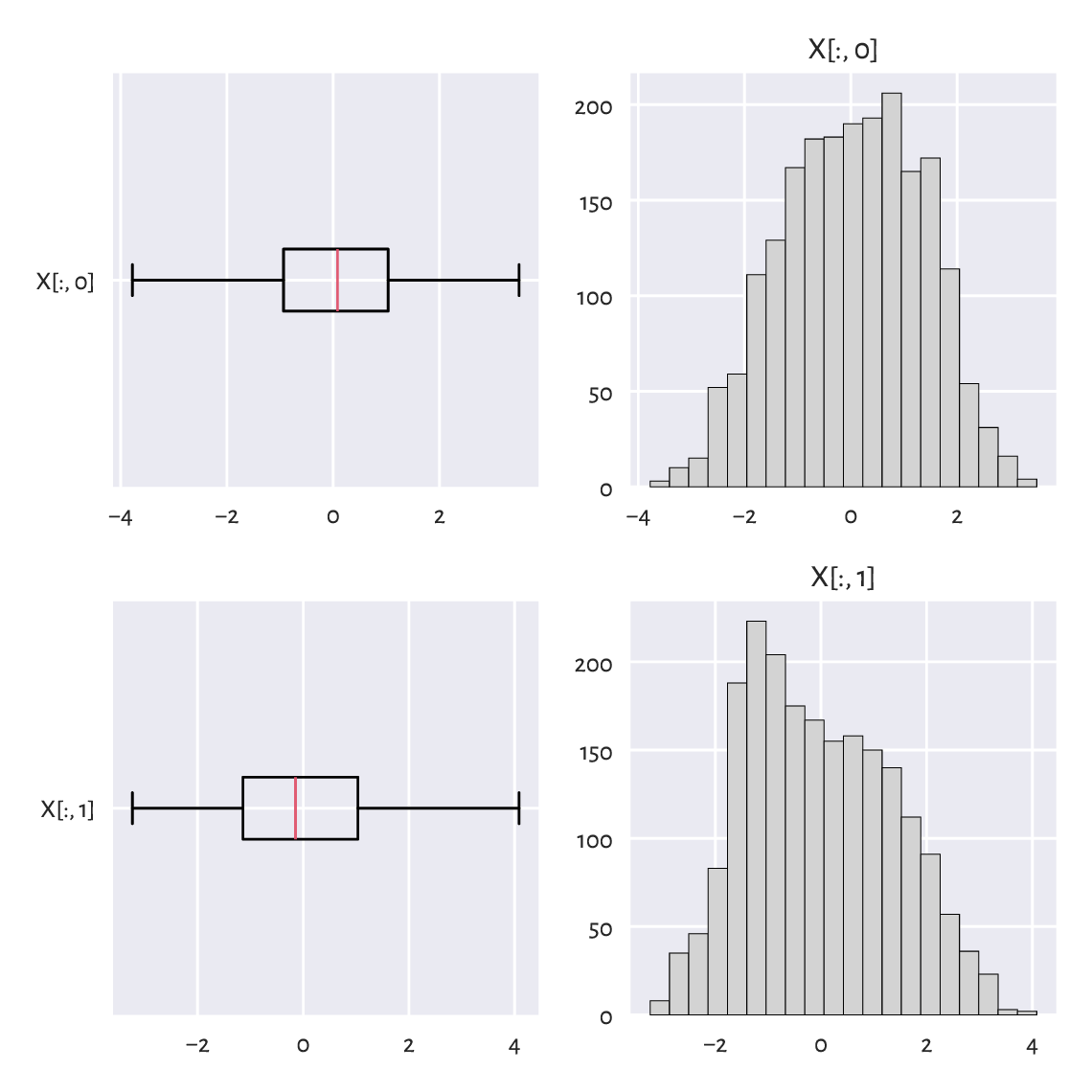
Figure 15.4 One-dimensional projections of the blobs1 dataset.

There is nothing suspicious here. Or is there?

The scatter plot in Figure 15.5 reveals that the data consist of two well-separable blobs:

plt.plot(X[:, 0], X[:, 1], "o")
plt.axis("equal")
plt.show()

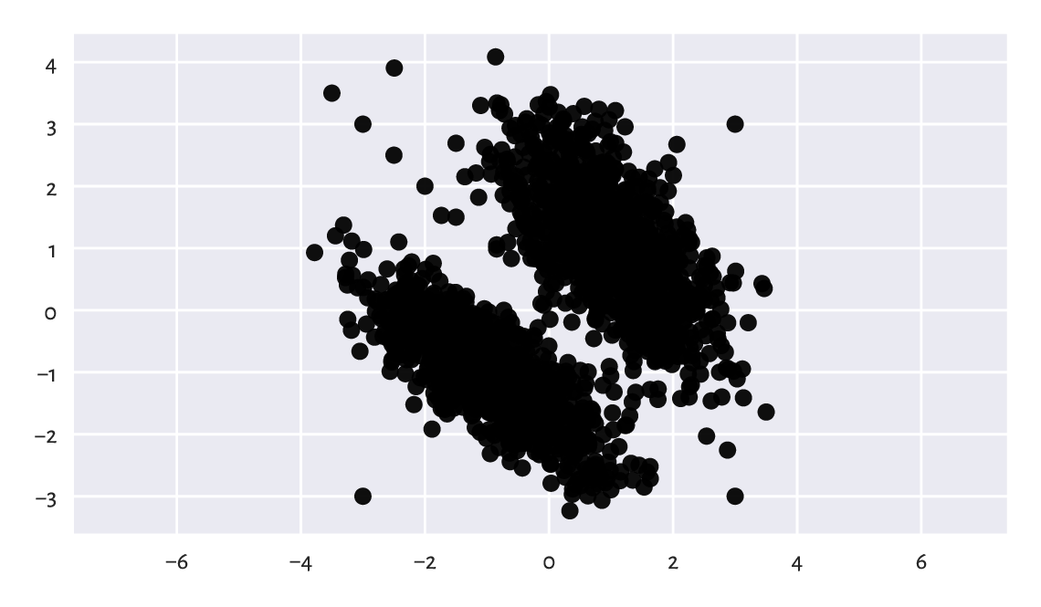
Figure 15.5 Scatter plot of the blobs1 dataset.

There are a few observations that we might mark as outliers. The truth is that yours truly injected eight junk points at the very end of the dataset. Ha.

X[-8:, :]
## array([[-3. ,  3. ],
##        [ 3. ,  3. ],
##        [ 3. , -3. ],
##        [-3. , -3. ],
##        [-3.5,  3.5],
##        [-2.5,  2.5],
##        [-2. ,  2. ],
##        [-1.5,  1.5]])

Handling multidimensional data requires slightly more sophisticated methods; see, e.g., [2]. A straightforward approach is to check if there are any points within an observation’s radius of some assumed size \(r>0\). If that is not the case, we may consider it an outlier. This is a variation on the aforementioned unidimensional density estimation approach[4].

Example 15.11

Consider the following code chunk:

t = scipy.spatial.KDTree(X)
n = t.query_ball_point(X, 0.2)  # r=0.2 (radius) – play with it yourself
c = np.array(pd.Series(n).str.len())
c[[0, 1, -2, -1]]  # preview
## array([42, 30,  1,  1])

c[i] gives the number of points within X[i, :]’s \(r\)-radius (with respect to the Euclidean distance), including the point itself. Consequently, c[i]==1 denotes a potential outlier; see Figure 15.6 for an illustration.

plt.plot(X[c > 1, 0], X[c > 1, 1], "o", label="normal point")
plt.plot(X[c == 1, 0], X[c == 1, 1], "v", label="outlier")
plt.axis("equal")
plt.legend()
plt.show()

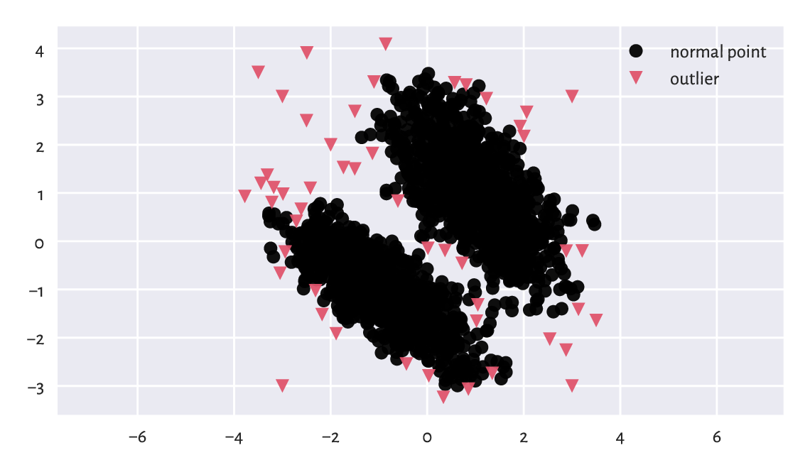
Figure 15.6 Outlier detection based on a fixed-radius search for the blobs1 dataset.

15.5. Exercises

Exercise 15.12

How can missing values be represented in numpy and pandas?

Exercise 15.13

Explain some basic strategies for dealing with missing values in numeric vectors.

Exercise 15.14

Why we ought to be very explicit about the way we handle missing and other suspicious data? Is it advisable to mark as missing (or remove completely) the observations that we dislike or otherwise deem inappropriate, controversial, dangerous, incompatible with our political views, etc.?

Exercise 15.15

Is replacing missing values with the sample arithmetic mean for income data (as in, e.g., the uk_income_simulated_2020 dataset) a sensible strategy?

Exercise 15.16

What are the differences between data missing completely at random, missing at random, and missing not at random?

Exercise 15.17

List some strategies for dealing with data that might contain outliers.

---

[1]

(*) The R environment, on the other hand, supports missing values out-of-the-box.

[2]

On the other hand, if we want to infer from small datasets, we should ask ourselves whether this is a good idea at all… It might be better to refrain from any data analysis than to come up with conclusions that are likely to be unjustified.

[3]

This is an instance of a kernel density estimator, with the simplest kernel: a rectangular one.

[4]

(**) We can easily normalise the outputs to get a true 2D kernel density estimator, but multivariate statistics is beyond the scope of this course. In particular, that data might have fixed marginal distributions (projections onto 1D) but their multidimensional images might be very different is beautifully described by the copula theory [69].