5. Processing unidimensional data

This open-access textbook is, and will remain, freely available for everyone’s enjoyment (also in PDF; a paper copy can also be ordered). It is a non-profit project. Although available online, it is a whole course, and should be read from the beginning to the end. Refer to the Preface for general introductory remarks. Any bug/typo reports/fixes are appreciated. Make sure to check out Deep R Programming [36] too.

Seldom will our datasets bring valid and valuable insights out of the box. The ones we are using for illustrational purposes in the first part of our book have already been curated. After all, it is an introductory course. We need to build the necessary skills up slowly, minding not to overwhelm the tireless reader with too much information all at once. We learn simple things first, learn them well, and then we move to more complex matters with a healthy level of confidence.

In real life, various data cleansing and feature engineering techniques will need to be applied. Most of them are based on the simple operations on vectors that we cover in this chapter:

• summarising data (for example, computing the median or sum),

• transforming values (applying mathematical operations on each element, such as subtracting a scalar or taking the natural logarithm),

• filtering (selecting or removing observations that meet specific criteria, e.g., those that are larger than the arithmetic mean ± 3 standard deviations).

Important

Chapter 10 will be applying the same operations on individual data frame columns.

5.1. Aggregating numeric data

Recall that in the previous chapter, we discussed the heights and income datasets whose histograms we gave in Figure 4.2 and Figure 4.3, respectively. Such graphical summaries are based on binned data. They provide us with snapshots of how much probability mass is allocated in different parts of the data domain.

Instead of dealing with large datasets, we obtained a few counts. The process of binning and its textual or visual depictions is valuable in determining whether the distribution is unimodal or multimodal, skewed or symmetric around some point, what range of values contains most of the observations, and how small or large extreme values are.

Too fine a level of information granularity may sometimes be overwhelming. Besides, revealing too much might not be a clever idea for privacy or confidentiality reasons[1]. Consequently, we might be interested in even more coarse descriptions: data aggregates which reduce the whole dataset into a single number reflecting some of its characteristics. Such summaries can provide us with a kind of bird’s-eye view of some of the dataset’s aspects.

In this part, we discuss a few noteworthy measures of:

• location; e.g., central tendency measures such as the arithmetic mean and median;

• dispersion; e.g., standard deviation and interquartile range;

• distribution shape; e.g., skewness.

We also introduce box-and-whisker plots.

5.1.1. Measures of location

5.1.1.1. Arithmetic mean and median

Two main measures of central tendency are:

• the arithmetic mean (sometimes for simplicity called the average or simply the mean), defined as the sum of all observations divided by the sample size:

  \[ \bar{x} = \frac{(x_1+x_2+\dots+x_n)}{n} = \frac{1}{n} \sum_{i=1}^n x_i, \]

• the median, being the middle value in a sorted version of the sample if its length is odd, or the arithmetic mean of the two middle values otherwise:

  \[ m = \left\{ \begin{array}{ll} x_{((n+1)/2)} & \text{if }n\text{ is odd},\\ \frac{x_{(n/2)}+x_{(n/2+1)}}{2} & \text{if }n\text{ is even}. \end{array} \right. \]

They can be computed using the numpy.mean and numpy.median functions.

heights = np.genfromtxt("https://raw.githubusercontent.com/gagolews/" +
    "teaching-data/master/marek/nhanes_adult_female_height_2020.txt")
np.mean(heights), np.median(heights)
## (160.13679222932953, 160.1)
income = np.genfromtxt("https://raw.githubusercontent.com/gagolews/" +
    "teaching-data/master/marek/uk_income_simulated_2020.txt")
np.mean(income), np.median(income)
## (35779.994, 30042.0)

Let’s underline what follows:

• for symmetric distributions, the arithmetic mean and the median are expected to be more or less equal;

• for skewed distributions, the arithmetic mean will be biased towards the heavier tail.

Exercise 5.1

Get the arithmetic mean and median for the 37_pzu_warsaw_marathon_mins dataset mentioned in Chapter 4.

Exercise 5.2

(*) Write a function that computes the median based on its mathematical definition and numpy.sort.

Note

(*) Technically, the arithmetic mean can also be computed using the mean method for the numpy.ndarray class. It will sometimes be the case that we have many ways to perform the same operation. We can even compose it manually using the sum function. Thus, all the following expressions are equivalent:

print(
    np.mean(income),
    income.mean(),
    np.sum(income)/len(income),
    income.sum()/income.shape[0]
)
## 35779.994 35779.994 35779.994 35779.994

Unfortunately, the median method for vectors is not available. As functions are more universal in numpy, we prefer sticking with them.

5.1.1.2. Sensitive to outliers vs robust

The arithmetic mean is strongly influenced by very large or very small observations which, in some contexts, we might refer to as outliers; see Section 15.4. Let’s invite a billionaire to swim in our income stream and check how the mean changes:

income2 = np.append(income, [1_000_000_000])
print(np.mean(income), np.mean(income2))
## 35779.994 1034745.2487512487

Comparing this new result to the previous one, oh we all feel much richer now, don’t we? In fact, the arithmetic mean reflects the income each of us would get if all the wealth were gathered inside a single Santa Claus’s (Robin Hood’s or Joseph Stalin’s) sack and then distributed equally amongst all of us. A noble idea provided that everyone contributes equally to the society which, sadly, is not the case.

On the other hand, the median is the value such that 50% of the observations are less than or equal to it and 50% of the remaining ones are not less than it. Hence, it is not at all sensitive to most of the data points on both the left and the right side of the distribution:

print(np.median(income), np.median(income2))
## 30042.0 30076.0

We cannot generally say that one measure is preferred to the other. It depends on the context (the nature of data, the requirements, etc.). Certainly, for symmetrical distributions with no outliers (e.g., heights), the mean will be better as it uses all data (and its efficiency can be proven for certain statistical models). For skewed distributions (e.g., income), the median has a nice interpretation, as it gives the value in the middle of the ordered sample. Remember that these data summaries allow us to look at a single data aspect only, and there can be many different, valid perspectives. The reality is complex.

5.1.1.3. Sample quantiles

Quantiles generalise the notion of the sample median and of the inverse of the empirical cumulative distribution function (Section 4.3.8). They provide us with the value that is not exceeded by the elements in a given sample with a predefined probability. Before proceeding with their formal definition, which is quite technical, let’s point out that for larger sample sizes, we have the following rule of thumb.

Important

For any \(p\) between 0 and 1, the \(p\)-quantile, denoted \(q_p\), is a value dividing the sample in such a way that approximately \(100p\%\) of observations are not greater than \(q_p\), and the remaining c. \(100(1-p)\%\) are not less than \(q_p\).

Quantiles appear under many different names, but they all refer to the same concept. In particular, we can speak about the \(100p\)-th percentiles, e.g., the 0.5-quantile is the same as the 50th percentile. Furthermore:

• 0-quantile (\(q_0\)) is the minimum (also: numpy.min),

• 0.25-quantile (\(q_{0.25}\)) equals to the first quartile (denoted \(Q_1\)),

• 0.5-quantile (\(q_{0.5}\)) is the second quartile a.k.a. median (denoted \(Q_2\) or \(m\)),

• 0.75-quantile (\(q_{0.75}\)) is the third quartile (denoted \(Q_3\)),

• 1.0-quantile (\(q_{1}\)) is the maximum (also: numpy.max).

Here are these five aggregates for our two example datasets:

np.quantile(heights, [0, 0.25, 0.5, 0.75, 1])
## array([131.1, 155.3, 160.1, 164.8, 189.3])
np.quantile(income,  [0, 0.25, 0.5, 0.75, 1])
## array([  5750.  ,  20669.75,  30042.  ,  44123.75, 199969.  ])

Example 5.3

Let’s print the aggregates neatly using f-strings; see Section 2.1.3.1:

wh = [0, 0.25, 0.5, 0.75, 1]
qheights = np.quantile(heights, wh)
qincome  = np.quantile(income, wh)
print("          heights     income")
for i in range(len(wh)):
    print(f"q_{wh[i]:<4g} {qheights[i]:10.2f} {qincome[i]:10.2f}")
##           heights     income
## q_0        131.10    5750.00
## q_0.25     155.30   20669.75
## q_0.5      160.10   30042.00
## q_0.75     164.80   44123.75
## q_1        189.30  199969.00

Exercise 5.4

What is the income bracket for 95% of the most typical UK taxpayers? In other words, determine the 2.5th and 97.5th percentiles.

Exercise 5.5

Compute the midrange of income and heights, being the arithmetic mean of the minimum and the maximum (this measure is extremely sensitive to outliers).

Note

(*) As we do not like the approximately part in the above “asymptotic definition”, in this course, we shall assume that for any \(p\in[0, 1]\), the \(p\)-quantile is given by:

\[ q_p = x_{(\lfloor k\rfloor)} + (k-\lfloor k\rfloor) (x_{(\lfloor k\rfloor+1)}-x_{(\lfloor k\rfloor)}), \]

where \(k=(n-1)p+1\) and \(\lfloor k\rfloor\) is the floor function, i.e., the greatest integer less than or equal to \(k\) (e.g., \(\lfloor 2.0\rfloor=\lfloor 2.001\rfloor=\lfloor 2.999\rfloor=2\), \(\lfloor 3.0\rfloor=\lfloor 3.999\rfloor=3\), \(\lfloor -3.0\rfloor=\lfloor -2.999\rfloor=\lfloor -2.001\rfloor=-3\), and \(\lfloor -2.0\rfloor=\lfloor -1.001\rfloor=-2\)).

\(q_p\) is a function that linearly interpolates between the points featuring the consecutive order statistics, \(((k - 1) / (n - 1), x_{(k)})\) for \(k=1,\dots,n\). For instance, for \(n=5\), we connect the points \((0, x_{(1)})\), \((0.25, x_{(2)})\), \((0.5, x_{(3)})\), \((0.75, x_{(4)})\), \((1, x_{(5)})\). For \(n=6\), we do the same for \((0, x_{(1)})\), \((0.2, x_{(2)})\), \((0.4, x_{(3)})\), \((0.6, x_{(4)})\), \((0.8, x_{(5)})\), \((1, x_{(6)})\); see Figure 5.1.

Notice that for \(p=0.5\) we get the median regardless of whether \(n\) is even or not.

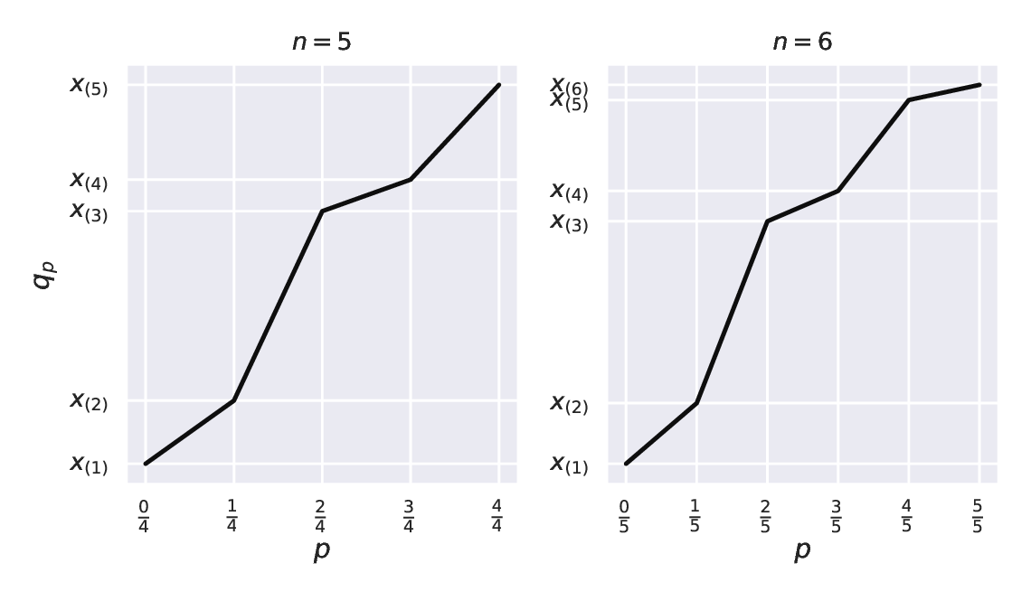
Figure 5.1 \(q_p\) as a function of \(p\) for example vectors of length 5 (left subfigure) and 6 (right).

Note

(**) There are many possible definitions of quantiles used in statistical software packages; see the method argument to numpy.quantile. They were nicely summarised in [56] as well as in the corresponding Wikipedia article. They are all approximately equivalent for large sample sizes (i.e., asymptotically), but the best practice is to be explicit about which variant we are using in the computations when reporting data analysis results. Accordingly, in our case, we say that we are relying on the type-7 quantiles as described in [56]; see also [47].

In fact, simply mentioning that our computations are done with numpy version 1.xx (as specified in Section 1.4) implicitly implies that the default method parameters are used everywhere, unless otherwise stated. In many contexts, that is good enough.

5.1.2. Measures of dispersion

Measures of central tendency quantify the location of the most typical value (whatever that means, and we already know it is complicated). That of dispersion (spread), on the other hand, will tell us how much variability or diversity is in our data. After all, when we say that the height of a group of people is 160 cm (on average) ± 14 cm (here, 2 standard deviations), the latter piece of information is a valuable addition (and is very different from the imaginary ± 4 cm case).

Some degree of variability might be welcome in certain contexts, and can be disastrous in others. A bolt factory should keep the variance of the fasteners’ diameters as low as possible: this is how we define quality products (assuming that they all meet, on average, the required specification). Nevertheless, too much diversity in human behaviour, where everyone feels that they are special, is not really sustainable (but lack thereof would be extremely boring).

Let’s explore the different ways in which we can quantify this data aspect.

5.1.2.1. Standard deviation (and variance)

The standard deviation[2], is the root mean square distance to the arithmetic mean:

\[ s = \sqrt{ \frac{ (x_1-\bar{x})^2 + (x_2-\bar{x})^2 + \dots + (x_n-\bar{x})^2 }{n} } = \sqrt{ \frac{1}{n} \sum_{i=1}^n (x_i-\bar{x})^2. } \]

Let’s compute it with numpy:

np.std(heights), np.std(income)
## (7.062021850008261, 22888.77122437908)

The standard deviation quantifies the typical amount of spread around the arithmetic mean. It is overall adequate for making comparisons across different samples measuring similar things (e.g., heights of males vs of females, incomes in the UK vs in South Africa).

However, without further assumptions, it can be difficult to express the meaning of a particular value of \(s\): for instance, the statement that the standard deviation of income is £22 900 is hard to interpret. This measure makes therefore most sense for data distributions that are symmetric around the mean.

Note

(*) For bell-shaped data such as heights (more precisely: for normally-distributed samples; see the next chapter), we sometimes report \(\bar{x}\pm 2s\). By the so-called \(2\sigma\) rule, the theoretical expectancy is that roughly 95% of data points fall into the \([\bar{x}-2s, \bar{x}+2s]\) interval.

Further, the variance is the square of the standard deviation, \(s^2\). Mind that if data are expressed in centimetres, then the variance is in centimetres squared, which is not very intuitive. The standard deviation does not have this drawback. For many reasons, mathematicians find the square root in the definition of \(s\) annoying, though; it is why we will come across the \(s^2\) measure every now and then too.

5.1.2.2. Interquartile range

The interquartile range (IQR) is another popular way to quantify data dispersion. It is defined as the difference between the third and the first quartile:

\[ \mathrm{IQR} = q_{0.75}-q_{0.25} = Q_3-Q_1. \]

Computing it is effortless:

np.quantile(heights, 0.75) - np.quantile(heights, 0.25)
## 9.5
np.quantile(income, 0.75) - np.quantile(income, 0.25)
## 23454.0

The IQR has an appealing interpretation: it is the range comprised of the 50% most typical values. It is a quite robust measure, as it ignores the 25% smallest and 25% largest observations. Standard deviation, on the other hand, is much more sensitive to outliers.

Furthermore, by range (or support) we will mean a measure based on extremal quantiles: it is the difference between the maximal and minimal observation.

5.1.3. Measures of shape

From a histogram, we can easily read whether a dataset is symmetric or skewed. It turns out that such a data characteristic can be easily quantified. Namely, the skewness is given by:

\[ g = \frac{ \frac{1}{n}\sum_{i=1}^n (x_i-\bar{x})^3 }{ \left(\sqrt{\frac{1}{n}\sum_{i=1}^n (x_i-\bar{x})^2}\right)^3 }. \]

For symmetric distributions, skewness is approximately zero. Positive and negative skewness indicates a heavier right and left tail, respectively.

For example, heights are an instance of an almost-symmetric distribution:

import scipy.stats
scipy.stats.skew(heights)
## 0.0811184528074054

and income is right-skewed:

scipy.stats.skew(income)
## 1.9768735693998942

Note

(*) It is worth stressing that \(g>0\) does not necessarily imply that the sample mean is greater than the median. As an alternative measure of skewness, the practitioners sometimes use:

\[ g'=\frac{\bar{x}-m}{s}. \]

Yule’s coefficient is an example of a robust skewness measure:

\[ g''=\frac{Q_3+Q_1-2m}{Q_3-Q_1}. \]

The computation thereof on our example datasets is left as an exercise.

Furthermore, kurtosis (Fisher’s excess kurtosis) describes whether an empirical distribution is heavy- or thin-tailed; compare scipy.stats.kurtosis.

5.1.4. Box (and whisker) plots

A box-and-whisker plot (box plot for short) depicts many noteworthy features of a data sample all at the same time.

plt.subplot(2, 1, 1)  # two rows, one column; the first subplot
plt.boxplot(heights, vert=False)
plt.yticks([1], ["heights"])  # label at y=1
plt.subplot(2, 1, 2)  # two rows, one column; the second subplot
plt.boxplot(income, vert=False)
plt.yticks([1], ["income"])  # label at y=1
plt.show()

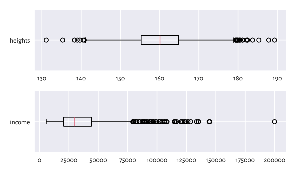
Figure 5.2 Example box plots.

Each box plot (compare Figure 5.2) consists of:

• the box, which spans between the first and the third quartile:

  • the median is clearly marked by a vertical bar inside the box;

  • the width of the box corresponds to the IQR;

• the whiskers, which span[3] between:

  • the smallest observation (the minimum) or \(Q_1-1.5 \mathrm{IQR}\) (the left side of the box minus 3/2 of its width), whichever is larger, and

  • the largest observation (the maximum) or \(Q_3+1.5 \mathrm{IQR}\) (the right side of the box plus 3/2 of its width), whichever is smaller.

Additionally, all observations that are less than \(Q_1-1.5 \mathrm{IQR}\) (if any) or greater than \(Q_3+1.5 \mathrm{IQR}\) (if any) are separately marked.

Note

We are used to referring to the individually marked points as outliers, but it does not automatically mean there is anything anomalous about them. They are atypical in the sense that they are considerably farther away from the box. It might indicate some problems in data quality (e.g., when someone made a typo entering the data), but not necessarily. Actually, box plots are calibrated (via the nicely round magic constant 1.5) in such a way that we expect there to be no or only few outliers if the data are normally distributed. For skewed distributions, there will naturally be many outliers on either side; see Section 15.4 for more details.

Box plots are based solely on sample quantiles. Most statistical packages do not draw the arithmetic mean. If they do, it is marked with a distinctive symbol.

Exercise 5.6

Call matplotlib.pyplot.plot(numpy.mean(..data..), 0, "bX") to mark the arithmetic mean with a blue cross. Alternatively, pass showmeans=True (amongst others) to matplotlib.pyplot.boxplot.

Box plots are particularly beneficial for comparing data samples with each other (e.g., body measures of men and women separately), both in terms of the relative shift (location) as well as spread and skewness; see, e.g., Figure 12.1.

Example 5.7

(*) A violin plot, see Figure 5.3, represents a kernel density estimator, which is a smoothened version of a histogram; see Section 15.4.2.

plt.subplot(2, 1, 1)  # two rows, one column; the first subplot
plt.violinplot(heights, vert=False, showextrema=False)
plt.boxplot(heights, vert=False)
plt.yticks([1], ["heights"])
plt.subplot(2, 1, 2)  # two rows, one column; the second subplot
plt.violinplot(income, vert=False, showextrema=False)
plt.boxplot(income, vert=False)
plt.yticks([1], ["income"])
plt.show()

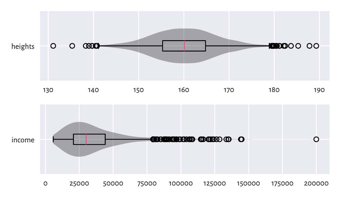
Figure 5.3 Example violin plots.

5.1.5. Other aggregation methods (*)

We said that the arithmetic mean is overly sensitive to extreme observations. The sample median is an example of a robust aggregate: it ignores all but 1–2 middle observations (we say it has a high breakdown point). Some measures of central tendency that are in-between the mean-median extreme include:

• trimmed means – the arithmetic mean of all the observations except several, say \(p\), smallest and greatest ones,

• winsorised means – the arithmetic mean with \(p\) smallest and \(p\) greatest observations replaced with the \((p+1)\)-th smallest and the \((p+1)\)-th greatest one, respectively.

The two other famous means are the geometric and harmonic ones. The former is more meaningful for averaging growth rates and speedups whilst the latter can be used for computing the average speed from speed measurements at sections of identical lengths; see also the notion of the F measure in Section 12.3.2. Also, the quadratic mean is featured in the definition of the standard deviation (it is the quadratic mean of the distances to the mean).

As far as spread measures are concerned, the interquartile range (IQR) is a robust statistic. If necessary, the standard deviation might be replaced with:

• mean absolute deviation from the mean: \(\frac{1}{n} \sum_{i=1}^n |x_i-\bar{x}|\),

• mean absolute deviation from the median: \(\frac{1}{n} \sum_{i=1}^n |x_i-m|\),

• median absolute deviation from the median: the median of \((|x_1-m|, |x_2-m|, \dots, |x_n-m|)\).

The coefficient of variation, being the standard deviation divided by the arithmetic mean, is an example of a relative (or normalised) spread measure. It can be appropriate for comparing data on different scales, as it is unitless (think how standard deviation changes when you convert between metres and centimetres).

The Gini index, widely used in economics, can also serve as a measure of relative dispersion, but assumes that all data points are nonnegative:

\[ G = \frac{ \sum_{i=1}^{n} \sum_{j=1}^n |x_i-x_j| }{ 2 (n-1)n\, \bar{x} } = \frac{ \sum_{i=1}^{n} (n-2i+1) x_{(n-i+1)} }{ (n-1) \sum_{i=1}^n x_i }. \]

It is normalised so that it takes values in the unit interval. An index of 0 reflects the situation where all values in a sample are the same (0 variance; perfect equality). If there is a single entity in possession of all the “wealth”, and the remaining ones are 0, then the index is equal to 1.

For a more generic (algebraic) treatment of aggregation functions for unidimensional data; see, e.g., [13, 32, 33, 45]. Some measures might be preferred under certain (often strict) assumptions usually explored in a course on mathematical statistics, e.g., [41].

Overall, numerical aggregates can be used in cases where data are unimodal. For multimodal mixtures or data in groups, they should rather be applied to summarise each cluster/class separately; compare Chapter 12. Also, Chapter 8 will extend some of the summaries for the case of multidimensional data.

5.2. Vectorised mathematical functions

numpy, just like any other comprehensive numerical computing environment (e.g., R, GNU Octave, Scilab, and Julia), gives access to many mathematical functions:

• absolute value: numpy.abs,

• square and square root: numpy.square and numpy.sqrt, respectively,

• (natural) exponential function: numpy.exp,

• logarithms: numpy.log (the natural logarithm, i.e., base \(e\)) and numpy.log10 (base \(10\)),

• trigonometric functions: numpy.cos, numpy.sin, numpy.tan, etc., and their inverses: numpy.arccos, etc.

• rounding and truncating: numpy.round, numpy.floor, numpy.ceil, numpy.trunc.

Important

The classical handbook of mathematical functions and the (in)equalities related to them is [1]; see [73] for its updated version.

Each of the aforementioned functions is vectorised. Applying, say, \(f\), on a vector like \(\boldsymbol{x}=(x_1,\dots,x_n)\), we obtain a sequence of the same length with all elements appropriately transformed:

\[ f(\boldsymbol{x}) = (f(x_1), f(x_2), \dots, f(x_n)). \]

In other words, \(f\) operates element by element on the whole array. Vectorised operations are frequently used for making adjustments to data, e.g., as in Figure 6.8, where we discover that the logarithm of the UK incomes has a bell-shaped distribution.

Here is an example call to the vectorised version of the rounding function:

np.round([-3.249, -3.151, 2.49, 2.51, 3.49, 3.51], 1)
## array([-3.2, -3.2,  2.5,  2.5,  3.5,  3.5])

The input list has been automatically converted to a numpy vector.

Important

Thanks to the vectorised functions, our code is not only more readable, but also runs faster: we do not have to employ the generally slow Python-level while or for loops to traverse through each element in a given sequence.

5.2.1. Logarithms and exponential functions

Let’s list some well-known properties of the natural logarithm and its inverse, the exponential function. By convention, Euler’s number \(e \simeq 2.718\), \(\log x = \log_e x\), and \(\exp(x)=e^x\).

• \(\log 1 = 0\), \(\log e = 1\),

• \(\log x^y = y \log x\) and hence \(\log e^x = x\),

• \(\log (xy) = \log x + \log y\) and thus \(\log (x/y) = \log x - \log y\),

• \(e^0 = 1\), \(e^1=e\),

• \(e^{\log x} = x\),

• \(e^{x+y} = e^x e^y\) and so \(e^{x-y}=e^x / e^y\),

• \(e^{xy} = (e^x)^y\).

Logarithms are only defined for \(x > 0\). Both functions are strictly increasing. For \(x\ge 1\), the logarithm grows very slowly whereas the exponential function increases very rapidly; see Figure 5.4. In the limit as \(x \to 0\), we have that \(\log x \to -\infty\). On the other hand, \(e^x\to 0\) as \(x \to -\infty\).

plt.subplot(1, 2, 1)
x = np.linspace(np.exp(-2), np.exp(3), 1001)
plt.plot(x, np.log(x), label="$y=\\log x$")
plt.legend()
plt.subplot(1, 2, 2)
x = np.linspace(-2, 3, 1001)
plt.plot(x, np.exp(x), label="$y=\\exp(x)$")
plt.legend()
plt.show()

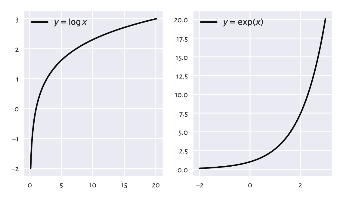
Figure 5.4 The natural logarithm (left) and the exponential function (right).

Logarithms of different bases and non-natural exponential functions are also available. In particular, when drawing plots, we used the base-10 logarithmic scales on the axes. We have \(\log_{10} x = \frac{\log x}{\log 10}\) and its inverse is \(10^x = e^{x \log 10}\). For example:

10.0**np.array([-1, 0, 1, 2])  # exponentiation; see below
## array([  0.1,   1. ,  10. , 100. ])
np.log10([-1, 0.01, 0.1, 1, 2, 5, 10, 100, 1000, 10000])
## <string>:1: RuntimeWarning: invalid value encountered in log10
## array([     nan, -2.     , -1.     ,  0.     ,  0.30103,  0.69897,
##         1.     ,  2.     ,  3.     ,  4.     ])

Take note of the warning and the not-a-number (NaN) generated.

Exercise 5.8

Check that when using the log-scale on the x-axis (plt.xscale("log")), the plot of the logarithm (of any base) is a straight line. Similarly, the log-scale on the y-axis (plt.yscale("log")) makes the exponential function linear.

5.2.2. Trigonometric functions

The trigonometric functions in numpy accept angles in radians. If \(x\) is the degree in angles, then to compute its cosine, we should instead write \(\cos (x \pi /180)\).

Figure 5.5 depicts the cosine and sine functions.

x = np.linspace(-2*np.pi, 4*np.pi, 1001)
plt.plot(x, np.cos(x), label="cos")  # black solid line (default style)
plt.plot(x, np.sin(x), 'r:', label="sin")  # red dotted line
plt.xticks(
    [-2*np.pi, -np.pi, 0, np.pi/2, np.pi, 3*np.pi/2, 2*np.pi, 4*np.pi],
    ["$-2\\pi$", "$-\\pi$", "$0$", "$\\pi/2$", "$\\pi$",
     "$3\\pi/2$", "$2\\pi$", "$4\\pi$"]
)
plt.legend()
plt.show()

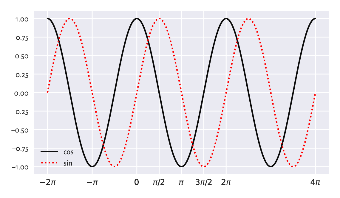
Figure 5.5 The cosine and the sine functions.

Some identities worth memorising, which we shall refer to later:

• \(\sin x = \cos(\pi/2 - x)\),

• \(\cos(-x) = \cos x\),

• \(\cos^2 x + \sin^2 x = 1\), where \(\cos^2 x = (\cos x)^2\),

• \(\cos(x+y) = \cos x \cos y - \sin x \sin y\),

• \(\cos(x-y) = \cos x \cos y + \sin x \sin y\).

5.3. Arithmetic operators

We can apply the standard binary (two-argument) arithmetic operators `+`, `-`, `*`, `/`, `**`, `%`, and `//` on vectors too. Beneath we discuss the possible cases of the operands’ lengths.

5.3.1. Vector-scalar case

Often, we will be referring to the binary operators in contexts where one operand is a vector and the other is a single value (scalar). For example:

np.array([-2, -1, 0, 1, 2, 3])**2
## array([4, 1, 0, 1, 4, 9])
(np.array([-2, -1, 0, 1, 2, 3])+2)/5
## array([0. , 0.2, 0.4, 0.6, 0.8, 1. ])

Each element was transformed (e.g., squared, divided by 5) and we got a vector of the same length in return. In these cases, the operators work just like the aforementioned vectorised mathematical functions.

Mathematically, we commonly assume that the scalar multiplication is performed in this way. In this book, we will also extend this behaviour to a scalar addition. Thus:

\[ c \boldsymbol{x} + t = (cx_1+t, cx_2+t, \dots, cx_n+t). \]

We will also become used to writing \((\boldsymbol{x}-t)/c\), which is equivalent to \((1/c) \boldsymbol{x} + (-t/c)\).

5.3.2. Application: Feature scaling

Vector-scalar operations and aggregation functions are the basis for the popular feature scalers that we discuss in the sequel:

• standardisation,

• min-max scaling and clipping,

• normalisation.

They can increase the interpretability of data points by bringing them onto a common, unitless scale. They might also be essential when computing pairwise distances between multidimensional points; see Section 8.4.

These transformations are of the form \(\boldsymbol{y}=c \boldsymbol{x}+t\), i.e., they are affine. We can interpret them geometrically as scaling (stretching or shrinking) and shifting (translating); see Figure 5.6 for an illustration.

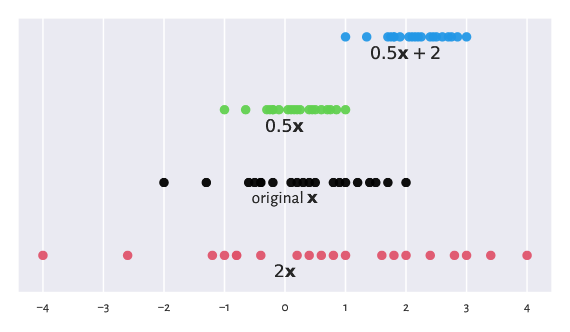
Figure 5.6 Scaled and shifted versions of an example vector.

Note

Let \(\boldsymbol{y}=c \boldsymbol{x}+t\) and let \(\bar{x}, \bar{y}, s_x, s_y\) denote the vectors’ arithmetic means and standard deviations. The following properties hold.

• The arithmetic mean is equivariant with respect to translation and scaling; we have \(\bar{y} = c \bar{x} + t\). This is also true for all the quantiles (including, of course, the median).

• The standard deviation is invariant to translations, and equivariant to scaling: \(s_y = c s_x\). The same happens for the interquartile range and the range.

As a byproduct, for the variance, we get \(s_y^2 = c^2 s_x^2\).

5.3.2.1. Standardisation and z-scores

A standardised version of a vector \(\boldsymbol{x}=(x_1,\dots,x_n)\) consists in subtracting, from each element, the sample arithmetic mean (which we call centring) and then dividing it by the standard deviation, i.e., \(\boldsymbol{z}=(\boldsymbol{x}-\bar{x})/s\). In other words, we transform each \(x_i\) to obtain:

\[ z_i = \frac{x_i-\bar{x}}{s}. \]

Consider again the female heights dataset:

heights[-5:]  # preview
## array([157. , 167.4, 159.6, 168.5, 147.8])

whose mean \(\bar{x}\) and standard deviation \(s\) are equal to:

np.mean(heights), np.std(heights)
## (160.13679222932953, 7.062021850008261)

With numpy, standardisation is as simple as applying two aggregation functions and two arithmetic operations:

heights_std = (heights-np.mean(heights))/np.std(heights)
heights_std[-5:]  # preview
## array([-0.44417764,  1.02848843, -0.07601113,  1.18425119, -1.74692071])

What we obtained is sometimes referred to as the z-scores. They are nicely interpretable:

• z-score of 0 corresponds to an observation equal to the sample mean (perfectly average);

• z-score of 1 is obtained for a datum 1 standard deviation above the mean;

• z-score of -2 means that it is a value 2 standard deviations below the mean;

and so forth.

Because of the way they emerge, the mean of the z-scores is always 0 and their standard deviation is 1 (up to a tiny numerical error, as usual; see Section 5.5.6):

np.mean(heights_std), np.std(heights_std)
## (1.8920872660373198e-15, 1.0)

Even though the original heights were measured in centimetres, the z-scores are unitless (centimetres divided by centimetres).

Important

Standardisation enables the comparison of measurements on different scales (think: height in centimetres vs weight in kilograms or apples vs oranges). It makes the most sense for bell-shaped distributions, in particular normally-distributed ones. Section 6.1.2 will introduce the \(2\sigma\) rule for the normal family (but not necessarily other models!). We will learn that we can expect that 95% of observations have z-scores between -2 and 2. Further, z-scores less than -3 and greater than 3 are highly unlikely.

Exercise 5.9

We have a patient whose height z-score is 1 and weight z-score is -1. How can we interpret this piece of information?

What about a patient whose weight z-score is 0 but BMI z-score is 2?

On a side note, sometimes we might be interested in performing some form of robust standardisation (e.g., for data with outliers or skewed). In such a case, we can replace the mean with the median and the standard deviation with the IQR.

5.3.2.2. Min-max scaling and clipping

A less frequently but still noteworthy transformation is called min-max scaling and involves subtracting the minimum and then dividing by the range, \((x-x_{(1)})/(x_{(n)}-x_{(1)})\).

x = np.array([-1.5, 0.5, 3.5, -1.33, 0.25, 0.8])
(x - np.min(x))/(np.max(x)-np.min(x))
## array([0.   , 0.4  , 1.   , 0.034, 0.35 , 0.46 ])

Here, the smallest value is mapped to 0 and the largest becomes equal to 1. Let’s stress that, in this context, 0.5 does not represent the value which is equal to the mean (unless we are incredibly lucky).

Also, clipping can be used to replace all values less than 0 with 0 and those greater than 1 with 1.

np.clip(x, 0, 1)
## array([0.  , 0.5 , 1.  , 0.  , 0.25, 0.8 ])

The function is, of course, flexible: another popular choice involves clipping to \([-1, 1]\). Note that this operation can also be composed by means of the vectorised pairwise minimum and maximum functions:

np.minimum(1, np.maximum(0, x))
## array([0.  , 0.5 , 1.  , 0.  , 0.25, 0.8 ])

5.3.2.3. Normalisation (\(l_2\); dividing by magnitude)

Normalisation is the scaling of a given vector so that it is of unit length. Usually, by length we mean the square root of the sum of squares, i.e., the Euclidean (\(l_2\)) norm also known as the magnitude:

\[ \| (x_1,\dots,x_n) \| = \sqrt{ x_1^2 + x_2^2 + \dots + x_n^2 } = \sqrt{ \sum_{i=1}^n x_i^2 }. \]

Its special case for \(n=2\) we know well from school: the length of a vector \((a,b)\) is \(\sqrt{a^2+b^2}\), e.g., \(\|(1, 2)\| = \sqrt{5} \simeq 2.236\). Also, we are advised to program our brains so that when we see \(\| \boldsymbol{x} \|^2\) next time, we immediately think of the sum of squares.

Consequently, a normalised vector:

\[ \frac{\boldsymbol{x}}{\| \boldsymbol{x} \|} = \left( \frac{x_1}{\| \boldsymbol{x} \|}, \frac{x_2}{\| \boldsymbol{x} \|}, \dots, \frac{x_n}{\| \boldsymbol{x} \|} \right), \]

can be determined via:

x = np.array([1, 5, -4, 2, 2.5])  # example vector
x/np.sqrt(np.sum(x**2))  # x divided by the Euclidean norm of x
## array([ 0.13834289,  0.69171446, -0.55337157,  0.27668579,  0.34585723])

Exercise 5.10

Normalisation is similar to standardisation if data are already centred (when the mean was subtracted). Show that we can obtain one from the other via the scaling by \(\sqrt{n}\).

Important

A common confusion is that normalisation is supposed to make data more normally distributed. This is not the case[4], as we only scale (stretch or shrink) the observations here.

5.3.2.4. Normalisation (\(l_1\); dividing by sum)

At other times, we might be interested in considering the Manhattan (\(l_1\)) norm:

\[ \| (x_1,\dots,x_n) \|_1 = |x_1| + |x_2| + \dots + |x_n| = \sum_{i=1}^n |x_i|, \]

being the sum of absolute values.

x / np.sum(np.abs(x))
## array([ 0.06896552,  0.34482759, -0.27586207,  0.13793103,  0.17241379])

\(l_1\) normalisation is frequently applied on vectors of nonnegative values, whose normalised versions can be interpreted as probabilities or proportions: values between 0 and 1 which sum to 1 (or, equivalently, 100%).

Example 5.11

Given some binned data:

c, b = np.histogram(heights, [-np.inf, 150, 160, 170, np.inf])
print(c)  # counts
## [ 306 1776 1773  366]

We can convert the counts to empirical probabilities:

p = c/np.sum(c)   # np.abs is not needed here
print(p)
## [0.07249467 0.42075338 0.42004264 0.08670931]

We did not apply numpy.abs because the values were already nonnegative.

5.3.3. Vector-vector case

We have been applying `*`, `+`, etc., so far on vectors and scalars only. All arithmetic operators can also be applied on two vectors of equal lengths. In such a case, they will act elementwisely: taking each element from the first operand and combining it with the corresponding element from the second argument:

np.array([2, 3, 4, 5]) * np.array([10, 100, 1000, 10000])
## array([   20,   300,  4000, 50000])

We see that the first element in the left operand (2) was multiplied by the first element in the right operand (10). Then, we multiplied 3 by 100 (the second corresponding elements), and so forth. Such a behaviour of the binary operators is inspired by the usual convention in vector algebra where applying \(+\) (or \(-\)) on \(\boldsymbol{x}=(x_1,\dots,x_n)\) and \(\boldsymbol{y}=(y_1,\dots,y_n)\) means exactly:

\[ \boldsymbol{x}+\boldsymbol{y} = (x_1+y_1, x_2+y_2, \dots, x_n+y_n). \]

Using other operators this way (elementwisely) is less standard in mathematics (for instance multiplication might denote the dot product), but in numpy it is really convenient.

Example 5.12

Let’s compute the value of the expression \(h = - (p_1\, \log p_1 + \dots + p_n\, \log p_n)\), i.e., \(h=-\sum_{i=1}^n p_i\, \log p_i\) (the entropy):

p = np.array([0.1, 0.3, 0.25, 0.15, 0.12, 0.08])  # example vector
-np.sum(p*np.log(p))
## 1.6790818544987114

It involves the use of a unary vectorised minus (change sign), an aggregation function (sum), a vectorised mathematical function (log), and an elementwise multiplication of two vectors of the same lengths.

Example 5.13

Assume we would like to plot two mathematical functions: the sine, \(f(x)= \sin x\), and a polynomial of degree 7, \(g(x) = x - x^3/6 + x^5/120 - x^7/5040\) for \(x\) in the interval \([-\pi, 3\pi/2]\). To do this, we can probe the values of \(f\) and \(g\) at sufficiently many points using the vectorised operations, and then use the matplotlib.pyplot.plot function to draw what we see in Figure 5.7.

x = np.linspace(-np.pi, 1.5*np.pi, 1001)  # many points in the said interval
yf = np.sin(x)
yg = x - x**3/6 + x**5/120 - x**7/5040
plt.plot(x, yf, 'k-', label="f(x)")  # black solid line
plt.plot(x, yg, 'r:', label="g(x)")  # red dotted line
plt.legend()
plt.show()

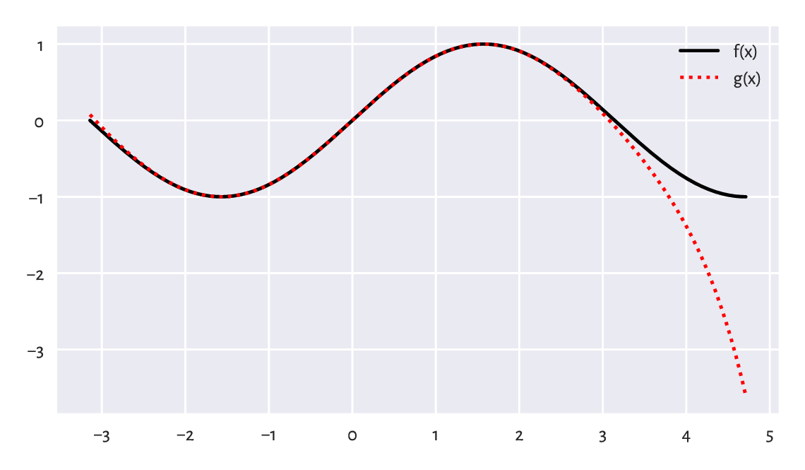
Figure 5.7 With vectorised functions, it is easy to generate plots like this one. We used different line styles so that the plot is readable also when printed in black and white.

Decreasing the number of points in x will reveal that the plotting function merely draws a series of straight-line segments. Computer graphics is essentially discrete.

Exercise 5.14

Using a single line of code, compute the vector of BMIs of all people in the nhanes_adult_female_height_2020 and nhanes_adult_female_weight_2020 datasets. It is assumed that the \(i\)-th elements therein both refer to the same person.

5.4. Indexing vectors

Recall from Section 3.2.1 and Section 3.2.2 that sequential objects in Python (lists, tuples, strings, ranges) support indexing with scalars and slices:

x = [10, 20, 30, 40, 50]
x[1]  # scalar index: extract
## 20
x[1:2]  # slice index: subset
## [20]

numpy vectors support two additional indexer types: integer and boolean sequences.

5.4.1. Integer indexing

First, indexing with a single integer extracts a particular element:

x = np.array([10, 20, 30, 40, 50])
x[0]   # the first
## 10
x[1]   # the second
## 20
x[-1]  # the last
## 50

Second, we can also use lists or vectors of integer indexes. They return a subvector with elements at the specified indexes:

x[ [0] ]
## array([10])
x[ [0, 1, -1, 0, 1, 0, 0] ]
## array([10, 20, 50, 10, 20, 10, 10])
x[ [] ]
## array([], dtype=int64)

Spaces between the square brackets were added only for readability, as x[[0]] looks slightly more obscure. (What are these double square brackets? Nah, it is a list inside the index operator.)

To return the vector with the elements except at the given indexes, we call the numpy.delete function. Its name is slightly misleading for the input vector is not modified in place.

np.delete(x, [0, -1])  # except the first and the last element
## array([20, 30, 40])

5.4.2. Logical indexing

Subsetting using a logical vector of the same length as the indexed vector is possible too:

x[ [True, False, True, True, False] ]
## array([10, 30, 40])

It returned the first, third, and fourth element (select the first, omit the second, choose the third, pick the fourth, skip the fifth).

Such type of indexing is particularly useful as a data filtering technique. Knowing that the relational vector operators `<`, `<=`, `==`, `!=`, `>=`, and `>` are performed elementwisely, just like `+`, `*`, etc., for instance:

x >= 30  # elementwise comparison
## array([False, False,  True,  True,  True])

we can write:

x[ x >= 30 ]  # indexing by a logical vector
## array([30, 40, 50])

to mean “select the elements in x which are not less than 30”. Of course, the indexed vector and the vector specifying the filter do not[5] have to be the same:

y = (x/10) % 2  # whatever
y  # equal to 0 if a number is a multiply of 10 times an even number
## array([1., 0., 1., 0., 1.])
x[ y == 0 ]
## array([20, 40])

Important

Sadly, if we wish to combine many logical vectors, we cannot use the and, or, and not operators. They are not vectorised (this is a limitation at the language level). Instead, in numpy, we use the `&`, `|`, and `~` operators. Alas, they have a higher order of precedence than `<`, `<=`, `==`, etc. Therefore, the bracketing of the comparisons is obligatory.

For example:

x[ (20 <= x) & (x <= 40) ]  # check what happens if we skip the brackets
## array([20, 30, 40])

means “elements in x between 20 and 40” (greater than or equal to 20 and less than or equal to 40). Also:

len(x[ (x < 15) | (x > 35) ])
## 3

computes the number of elements in x which are less than 15 or greater than 35 (are not between 15 and 35).

Exercise 5.15

Compute the BMIs only of the women whose height is between 150 and 170 cm.

5.4.3. Slicing

Just as with ordinary lists, slicing with `:` fetches the elements at indexes in a given range like from:to or from:to:by.

x[:3]  # the first three elements
## array([10, 20, 30])
x[::2]  # every second element
## array([10, 30, 50])
x[1:4]  # from the second (inclusive) to the fifth (exclusive)
## array([20, 30, 40])

Important

For efficiency reasons, slicing returns a view of existing data. It does not have to make an independent copy of the subsetted elements: by definition, sliced ranges are regular.

In other words, both x and its sliced version share the same memory. This is important when we apply operations which modify a given vector in place, such as the sort method that we mention in the sequel.

def zilchify(x):
    x[:] = 0  # re-sets all values in x

y = np.array([6, 4, 8, 5, 1, 3, 2, 9, 7])
zilchify(y[::2])  # modifies parts of y in place
y  # has changed
## array([0, 4, 0, 5, 0, 3, 0, 9, 0])

It zeroed every second element in y. On the other hand, indexing with an integer or logical vector always returns a copy.

zilchify(y[ [1, 3, 5, 7] ])  # modifies a new object and then forgets about it
y  # has not changed since the last modification
## array([0, 4, 0, 5, 0, 3, 0, 9, 0])

The original vector has not been modified, because we applied the function on a new (temporary) object. However, we note that compound operations such as += work differently, because setting elements at specific indexes is always possible:

y[ [0, -1] ] += 7  # the same as y[ [0, 7] ] = y[ [0, 7] ] + 7
y
## array([7, 4, 0, 5, 0, 3, 0, 9, 7])

5.5. Other operations

5.5.1. Cumulative sums and iterated differences

Recall that the `+` operator acts on two vectors elementwisely and that the numpy.sum function aggregates all values into a single one. We have a similar function, but vectorised in a slightly different fashion: numpy.cumsum returns the vector of cumulative sums:

np.cumsum([5, 3, -4, 1, 1, 3])
## array([5, 8, 4, 5, 6, 9])

It gave, in this order: the first element, the sum of the first two elements, the sum of the first three elements, …, the sum of all elements.

Iterated differences are a somewhat inverse operation:

np.diff([5, 8, 4, 5, 6, 9])
## array([ 3, -4,  1,  1,  3])

It returned the difference between the second and the first element, then the difference between the third and the second, and so forth. The resulting vector is one element shorter than the input one.

We often make use of cumulative sums and iterated differences when processing time series, e.g., stock exchange data (e.g., by how much the price changed since the previous day?; Section 16.3.1) or determining cumulative distribution functions (Section 4.3.8).

5.5.2. Sorting

The numpy.sort function returns a sorted copy of a given vector, i.e., determines the order statistics.

x = np.array([50, 30, 10, 40, 20, 30, 50])
np.sort(x)
## array([10, 20, 30, 30, 40, 50, 50])

The sort method, on the other hand, sorts the vector in place (and returns nothing).

x  # before
## array([50, 30, 10, 40, 20, 30, 50])
x.sort()
x  # after
## array([10, 20, 30, 30, 40, 50, 50])

Exercise 5.16

Readers concerned more with chaos than bringing order should give numpy.random.permutation a try: it shuffles the elements in a given vector.

5.5.3. Dealing with tied observations

Some statistical methods, especially for continuous data[6], assume that all observations in a vector are unique, i.e., there are no ties. In real life, however, some values might be recorded multiple times. For instance, two marathoners might finish their runs in exactly the same time, data can be rounded up to a certain number of fractional digits, or it just happens that observations are inherently integer. Therefore, we should be able to detect duplicated entries.

numpy.unique is a workhorse for dealing with tied observations.

x = np.array([40, 10, 20, 40, 40, 30, 20, 40, 50, 10, 10, 70, 30, 40, 30])
np.unique(x)
## array([10, 20, 30, 40, 50, 70])

It returned a sorted[7] version of a given vector with duplicates removed.

We can also get the corresponding counts:

np.unique(x, return_counts=True)  # returns a tuple of length 2
## (array([10, 20, 30, 40, 50, 70]), array([3, 2, 3, 5, 1, 1]))

It can help determine if all the values in a vector are unique:

np.all(np.unique(x, return_counts=True)[1] == 1)
## False

Exercise 5.17

Play with the return_index argument to numpy.unique. It permits pinpointing the indexes of the first occurrences of each unique value.

5.5.4. Determining the ordering permutation and ranking

numpy.argsort returns a sequence of indexes that lead to an ordered version of a given vector (i.e., an ordering permutation).

x = np.array([50, 30, 10, 40, 20, 30, 50])
np.argsort(x)
## array([2, 4, 5, 1, 3, 0, 6])

Which means that the smallest element is at index 2, then the second smallest is at index 4, the third smallest at index 1, etc. Therefore:

x[np.argsort(x)]
## array([10, 20, 30, 30, 40, 50, 50])

is equivalent to numpy.sort(x).

Note

(**) If there are tied observations in x, numpy.argsort(x, kind="stable") will use a stable sorting algorithm (timsort, a variant of mergesort), which guarantees that the ordering permutation is unique: tied elements are placed in the order of appearance.

Next, scipy.stats.rankdata returns a vector of ranks.

x = np.array([50, 30, 10, 40, 20, 30, 50])
scipy.stats.rankdata(x)
## array([6.5, 3.5, 1. , 5. , 2. , 3.5, 6.5])

Element 10 is the smallest (“the winner”, say, the quickest racer). Hence, it ranks first. The two tied elements equal to 30 are the third/fourth on the podium (ex aequo). Thus, they receive the average rank of 3.5. And so on.

On a side note, there are many methods in nonparametric statistics (where we do not make any particular assumptions about the underlying data distribution) that are based on ranks. In particular, Section 9.1.4 will cover the Spearman correlation coefficient.

Exercise 5.18

Consult the manual page of scipy.stats.rankdata and test various methods for dealing with ties.

Exercise 5.19

What is the interpretation of a rank divided by the length of the sample?

Note

(**) Calling numpy.argsort on a vector representing a permutation of indexes generates its inverse. In particular, np.argsort(np.argsort(x, kind="stable"))+1 is equivalent to scipy.stats.rankdata(x, method="ordinal").

5.5.5. Searching for certain indexes (argmin, argmax)

numpy.argmin and numpy.argmax return the index at which we can find the smallest and the largest observation in a given vector.

x = np.array([50, 30, 10, 40, 20, 30, 50])
np.argmin(x), np.argmax(x)
## (2, 0)

Using mathematical notation, the former is denoted by:

\[ i = \mathrm{arg}\min_j x_j, \]

and we read it as “let \(i\) be the index of the smallest element in the sequence”. Alternatively, it is the argument of the minimum, whenever:

\[ x_i = \min_j x_j, \]

i.e., the \(i\)-th element is the smallest.

If there are multiple minima or maxima, the leftmost index is returned.

We can use numpy.flatnonzero to fetch the indexes where a logical vector has elements equal to True (Section 11.1.2 mentions that a value equal to zero is treated as the logical False, and as True in all other cases). For example:

np.flatnonzero(x == np.max(x))
## array([0, 6])

It is a version of numpy.argmax that lets us decide what we would like to do with the tied maxima (there are two).

Exercise 5.20

Let x be a vector with possible ties. Create an expression that returns a randomly chosen index pinpointing one of the sample maxima.

5.5.6. Dealing with round-off and measurement errors

Mathematics tells us (the easy proof is left as an exercise for the reader) that a centred version of a given vector \(\boldsymbol{x}\), \(\boldsymbol{y} = \boldsymbol{x}-\bar{x}\), has the arithmetic mean of 0, i.e., \(\bar{y}=0\). Of course, it is also true on a computer. But is it?

heights_centred = (heights - np.mean(heights))
np.mean(heights_centred) == 0
## False

The average is actually equal to:

np.mean(heights_centred)
## 1.3359078775153175e-14

which is almost zero (0.0000000000000134), but not exactly zero (it is zero for an engineer, not a mathematician). We saw a similar result in Section 5.3.2, when we standardised a vector (which involves centring).

Important

All floating-point operations on a computer[8] (not only in Python) are performed with finite precision of 15–17 decimal digits.

We know it from school. For example, some fractions cannot be represented as decimals. When asked to add or multiply them, we will always have to apply some rounding that ultimately leads to precision loss. We know that \(1/3 + 1/3 + 1/3 = 1\), but using a decimal representation with one fractional digit, we get \(0.3+0.3+0.3=0.9\). With two digits of precision, we obtain \(0.33+0.33+0.33=0.99\). And so on. This sum will never be equal exactly to 1 when using a finite precision.

Note

Our data are often imprecise by nature. When asked about people’s heights, rarely will they provide a non-integer answer (assuming they know how tall they are and are not lying about it, but it is a different story). We will most likely get data rounded to 0 decimal digits. In our heights dataset, the precision is a bit higher:

heights[:6]  # preview
## array([160.2, 152.7, 161.2, 157.4, 154.6, 144.7])

But still, we expect there to be some inherent observational error.

Moreover, errors induced at one stage will propagate onto further operations. For instance, that the heights data are not necessarily accurate, makes their aggregates such as the mean approximate as well. Most often, the errors should more or less cancel out, but in extreme cases, they can lead to undesirable consequences (like for some model matrices in linear regression; see Section 9.2.9).

Exercise 5.21

Compute the BMIs of all females in the NHANES study. Determine their arithmetic mean. Compare it to the arithmetic mean computed for BMIs rounded to 1, 2, 3, 4, etc., decimal digits.

There is no reason to panic, though. The rule to remember is as follows.

Important

As the floating-point values are precise up to a few decimal digits, we must refrain from comparing them using the `==` operator, which tests for exact equality.

When a comparison is needed, we need to take some error margin \(\varepsilon > 0\) into account. Ideally, instead of testing x == y, we either inspect the absolute error:

\[ |x-y| \le \varepsilon, \]

or, assuming \(y\neq 0\), the relative error:

\[ \frac{|x-y|}{|y|} \le \varepsilon. \]

For instance, numpy.allclose(x, y) checks (by default) if for all corresponding elements in both vectors, we have numpy.abs(x-y) <= 1e-8 + 1e-5*numpy.abs(y), which is a combination of both tests.

np.allclose(np.mean(heights_centred), 0)
## True

To avoid sorrow surprises, even the testing of inequalities like x >= 0 should rather be performed as, say, x >= 1e-8.

Note

(*) Another problem is related to the fact that floats on a computer use the binary base, not the decimal one. Therefore, some fractional numbers that we believe to be representable exactly, require an infinite number of bits. As a consequence, they are subject to rounding.

0.1 + 0.1 + 0.1 == 0.3  # obviously
## False

This is because 0.1, 0.1+0.1+0.1, and 0.3 are literally represented as, respectively:

print(f"{0.1:.19f}, {0.1+0.1+0.1:.19f}, and {0.3:.19f}.")
## 0.1000000000000000056, 0.3000000000000000444, and 0.2999999999999999889.

A suggested introductory reference to the topic of numerical inaccuracies is [43]; see also [51, 59] for a more comprehensive treatment of numerical analysis.

5.5.7. Vectorising scalar operations with list comprehensions

List comprehensions of the form [ expression for name in iterable ] are part of base Python. They create lists based on transformed versions of individual elements in a given iterable object. Hence, they might work in cases where a task at hand cannot be solved by means of vectorised numpy functions.

For example, here is a way to generate the squares of a few positive natural numbers:

[ i**2 for i in range(1, 11) ]
## [1, 4, 9, 16, 25, 36, 49, 64, 81, 100]

The result can be passed to numpy.array to convert it to a vector. Further, given an example vector:

x = np.round(np.random.rand(9)*2-1, 2)
x
## array([ 0.86, -0.37, -0.63, -0.59,  0.14,  0.19,  0.93,  0.31,  0.5 ])

if we wish to filter out all elements that are not positive, we can write:

[ e for e in x if e > 0 ]
## [0.86, 0.14, 0.19, 0.93, 0.31, 0.5]

We can also use the ternary operator of the form x_true if cond else x_false to return either x_true or x_false depending on the truth value of cond.

e = -2
e**0.5 if e >= 0 else (-e)**0.5
## 1.4142135623730951

Combined with a list comprehension, we can write, for instance:

[ round(e**0.5 if e >= 0 else (-e)**0.5, 2) for e in x ]
## [0.93, 0.61, 0.79, 0.77, 0.37, 0.44, 0.96, 0.56, 0.71]

This gave the square root of absolute values.

There is also a tool which vectorises a scalar function so that it can be used on numpy vectors:

def clip01(x):
    """clip to the unit interval"""
    if x < 0:    return 0
    elif x > 1:  return 1
    else:        return x

clip01s = np.vectorize(clip01)  # returns a function object
clip01s([0.3, -1.2, 0.7, 4, 9])
## array([0.3, 0. , 0.7, 1. , 1. ])

Overall, vectorised numpy functions lead to faster, more readable code. However, if the corresponding operations are unavailable (e.g., string processing, reading many files), list comprehensions can serve as their reasonable replacement.

Exercise 5.22

Write equivalent versions of the above expressions using vectorised numpy functions. Moreover, implement them using base Python lists, the for loop and the list.append method (start from an empty list that will store the result). Use the timeit module to compare the run times of different approaches on large vectors.

5.6. Exercises

Exercise 5.23

What are some benefits of using a numpy vector over an ordinary Python list? What are the drawbacks?

Exercise 5.24

How can we interpret the possibly different values of the arithmetic mean, median, standard deviation, interquartile range, and skewness, when comparing between heights of men and women?

Exercise 5.25

There is something scientific and magical about numbers that make us approach them with some kind of respect. However, taking into account that there are many possible data aggregates, there is a risk that a party may be cherry-picking: report the value that portrays the analysed entity in a good or bad light, e.g., choose the mean instead of the median or vice versa. Is there anything that can be done about it?

Exercise 5.26

Even though, mathematically speaking, all measures can be computed on all data, it does not mean that it always makes sense to do so. For instance, some distributions will have skewness of 0. However, we should not automatically assume that they are delightfully symmetric and bell-shaped (e.g., this can be a bimodal distribution). We always ought to visualise our data. Give some examples of datasets where we need to be critical of the obtained aggregates.

Exercise 5.27

Give the mathematical definitions, use cases, and interpretations of standardisation, normalisation, and min-max scaling.

Exercise 5.28

How are numpy.log and numpy.exp related to each other? What about numpy.log vs numpy.log10, numpy.cumsum vs numpy.diff, numpy.min vs numpy.argmin, numpy.sort vs numpy.argsort, and scipy.stats.rankdata vs numpy.argsort?

Exercise 5.29

What is the difference between numpy.trunc, numpy.floor, numpy.ceil, and numpy.round?

Exercise 5.30

What happens when we apply `+` on two vectors of different lengths?

Exercise 5.31

List the four general ways to index a vector.

Exercise 5.32

What is wrong with the expression x[ x >= 0 and x <= 1 ], where x is a numeric vector? What about x[ x >= 0 & x <= 1 ]?

Exercise 5.33

What does it mean that slicing returns a view of existing data?

Exercise 5.34

Given a numeric vector x, for instance:

np.random.seed(123)
x = np.round(np.random.randn(20), 2)

perform what follows.

1. Print out all values in x that belong to the set \([-2,-1]\cup[1,2]\).

2. Print out the number and the fraction of nonnegative values in x.

3. Find the position (index) of the first value greater than 2.

4. Create two vectors xo and xe consisting of the items at odd and even indices, respectively.

5. Compute the range, i.e., the difference between the greatest and the smallest value.

6. Compute the midrange, i.e., the arithmetic mean of the maximum and the minimum.

7. Compute the mean of absolute values.

8. Find the values closest to and farthest away from 0.

9. Find the values closest to and farthest away from 2.

Exercise 5.35

Write a function to compute the \(k\)-winsorised mean, given a numeric vector x and \(k\le \frac{n-1}{2}\), i.e., the arithmetic mean of a version of x, where the \(k\) smallest and \(k\) greatest values were replaced by the \((k+1)\)-th smallest and greatest value, respectively.

Exercise 5.36

(**) Reflect on the famous saying: not everything that can be counted counts, and not everything that counts can be counted.

Exercise 5.37

(**) Being a data scientist can be a frustrating job, especially when you care for some causes. Reflect on: some things that count can be counted, but we will not count them because we ran over budget or because our stupid corporate manager simply doesn’t care.

Exercise 5.38

(**) Being a data scientist can be a frustrating job, especially when you care for the truth. Reflect on: some things that count can be counted, but we will not count them for some people might be offended or find it unpleasant.

Exercise 5.39

(**) Assume you were to become the benevolent dictator of a nation living on some remote island. How would you measure if your people are happy or not? Assume that you need to come up with three quantitative measures (key performance indicators). What would happen if your policy-making was solely focused on optimising those KPIs? What about the same problem but in the context your company and employees? Think about what can go wrong in other areas of life.

---

[1]

Nevertheless, we strongly advocate for all information of concern to the public to be openly available, so that experienced statisticians can put them to good use.

[2]

(**) We mean the one based on the so-called uncorrected for statistical bias version of the sample variance. We prefer it here for didactical reasons (simplicity, interpretability). Plus, it is the default one in numpy. Passing ddof=1 (delta degrees of freedom) to numpy.std will apply division by \(n-1\) instead of by \(n\) (we will note later that the std methods in pandas have it activated by default). When used as an estimator of the distribution’s standard deviation, the latter has slightly better statistical properties that we normally explore in a course on mathematical statistics, which this one is not.

[3]

The \(1.5 \mathrm{IQR}\) rule is the most popular in the statistical literature, but some plotting software may use different whisker ranges. See Section 15.4.1 for further discussion.

[4]

(*) A Box–Cox transformation [12] can help achieve this in some datasets. Chapter 6 will apply its particular case: it will turn out that the logarithm of incomes follow a normal distribution (hence, incomes follow a log-normal distribution). Generally, there is nothing “wrong” or “bad” about data’s not being normally-distributed. It is just a nice feature to have in certain contexts.

[5]

(*) The indexer is computed first, and its value is passed as an argument to the index operator. Python neither is a symbolic programming language, nor does it feature any nonstandard evaluation techniques. In other words, [...] does not care how the indexer was obtained.

[6]

Where, theoretically, the probability of obtaining a tie is equal to 0.

[7]

Later we will mention pandas.unique which lists the values in the order of appearance.

[8]

Double precision float64 format as defined by the IEEE Standard for Floating-Point Arithmetic (IEEE 754).