7. From uni- to multidimensional numeric data
This open-access textbook is, and will remain, freely available for everyone’s enjoyment (also in PDF; a paper copy can also be ordered). It is a non-profit project. Although available online, it is a whole course, and should be read from the beginning to the end. Refer to the Preface for general introductory remarks. Any bug/typo reports/fixes are appreciated. Make sure to check out Deep R Programming [36] too.
From the perspective of structured datasets, a vector often represents \(n\) independent measurements of the same quantitative property, e.g., heights of \(n\) different patients, incomes in \(n\) randomly chosen households, or finishing times of \(n\) marathoners. More generally, these are all instances of a bag of \(n\) points on the real line. By far[1], we should have become fairly fluent with the methods for processing such one-dimensional arrays.
Let’s increase the level of complexity by describing the \(n\) entities by \(m\) features, for any \(m\ge 1\). In other words, we will be dealing with \(n\) points in an \(m\)-dimensional space, \(\mathbb{R}^m\).
We can arrange all the observations in a table with \(n\) rows and \(m\) columns (just like in spreadsheets). We can represent it with numpy as a two-dimensional array which we will refer to as a matrix. Thanks to matrices, we can keep the \(n\) tuples of length \(m\) together in a single object (or \(m\) tuples of length \(n\), depending on how we want to look at them) and process them all at once. How convenient.
Important
Just like vectors, matrices were designed to store data of the same type. Chapter 10 will cover pandas data frames, which support mixed data types, e.g., numerical and categorical. Moreover, they let their rows and columns be named. pandas is built on top of numpy, and implements many recipes for the most popular data wrangling tasks. We, however, we would like to be able to tackle any computational problem. It is worth knowing that many data analysis and machine learning algorithms automatically convert numerical parts of data frames to matrices so that numpy can do most of the mathematical heavy lifting.
7.1. Creating matrices
7.1.1. Reading CSV files
Tabular data are often stored and distributed in a very portable plain-text format called CSV (comma-separated values) or one of its variants. We can read them easily with numpy.genfromtxt (or later with pandas.read_csv).
body = np.genfromtxt("https://raw.githubusercontent.com/gagolews/" +
    "teaching-data/master/marek/nhanes_adult_female_bmx_2020.csv",
    delimiter=",")[1:, :]  # skip the first row (column names)
The file specifies column names in the first non-comment line (we suggest inspecting it in a web browser). Therefore, we had to omit it manually (more on matrix indexing later). Here is a preview of the first few rows:
body[:6, :]  # the first six rows, all columns
## array([[ 97.1, 160.2,  34.7,  40.8,  35.8, 126.1, 117.9],
##        [ 91.1, 152.7,  33.5,  33. ,  38.5, 125.5, 103.1],
##        [ 73. , 161.2,  37.4,  38. ,  31.8, 106.2,  92. ],
##        [ 61.7, 157.4,  38. ,  34.7,  29. , 101. ,  90.5],
##        [ 55.4, 154.6,  34.6,  34. ,  28.3,  92.5,  73.2],
##        [ 62. , 144.7,  32.5,  34.2,  29.8, 106.7,  84.8]])
It is an excerpt from the National Health and Nutrition Examination Survey (NHANES), where the consecutive columns give seven body measurements of adult females:
body_columns = np.array([
    "weight (kg)",
    "standing height (cm)",   # we know `heights` from the previous chapters
    "upper arm len. (cm)",
    "upper leg len. (cm)",
    "arm circ. (cm)",
    "hip circ. (cm)",
    "waist circ. (cm)",
])
We noted the column names down as numpy matrices give no means for storing column labels. It is only a minor inconvenience.
body is a numpy array:
type(body)  # class of this object
## <class 'numpy.ndarray'>
but this time it is a two-dimensional one:
body.ndim  # number of dimensions
## 2
which means that its shape slot is now a tuple of length two:
body.shape
## (4221, 7)
We obtained the total number of rows and columns, respectively.
7.1.2. Enumerating elements
numpy.array can take a sequence of vector-like objects of the same lengths specifying consecutive rows of a matrix. For example:
np.array([  # list of lists
    [ 1,  2,  3,  4 ],  # the first row
    [ 5,  6,  7,  8 ],  # the second row
    [ 9, 10, 11, 12 ]   # the third row
])
## array([[ 1,  2,  3,  4],
##        [ 5,  6,  7,  8],
##        [ 9, 10, 11, 12]])
gives a \(3\times 4\) (3-by-4) matrix. Next:
np.array([ [1], [2], [3] ])
## array([[1],
##        [2],
##        [3]])
yields a \(3\times 1\) array. Such two-dimensional arrays with one column will be referred to as column vectors (they are matrices still). Moreover:
np.array([ [1, 2, 3, 4] ])
## array([[1, 2, 3, 4]])
produces a \(1\times 4\) array (a row vector).
Note
An ordinary vector (a unidimensional array) only displays a single pair of square brackets:
np.array([1, 2, 3, 4])
## array([1, 2, 3, 4])
7.1.3. Repeating arrays
The previously-mentioned numpy.tile and numpy.repeat can also generate some nice matrices. For instance:
np.repeat([[1, 2, 3, 4]], 3, axis=0)  # over the first axis
## array([[1, 2, 3, 4],
##        [1, 2, 3, 4],
##        [1, 2, 3, 4]])
repeats a row vector rowwisely, i.e., over the first axis (0). Replicating a column vector columnwisely is possible as well:
np.repeat([[1], [2], [3]], 4, axis=1)  # over the second axis
## array([[1, 1, 1, 1],
##        [2, 2, 2, 2],
##        [3, 3, 3, 3]])
Generate matrices of the following kinds:
7.1.4. Stacking arrays
numpy.column_stack and numpy.vstack take a tuple of array-like objects and bind them column- or rowwisely to form a new matrix:
np.column_stack(([10, 20], [30, 40], [50, 60]))  # a tuple of lists
## array([[10, 30, 50],
##        [20, 40, 60]])
np.vstack(([10, 20], [30, 40], [50, 60]))
## array([[10, 20],
##        [30, 40],
##        [50, 60]])
np.column_stack((
    np.vstack(([10, 20], [30, 40], [50, 60])),
    [70, 80, 90]
))
## array([[10, 20, 70],
##        [30, 40, 80],
##        [50, 60, 90]])
Note the double round brackets: we called these functions on tuples.
Perform similar operations using numpy.append, numpy.hstack, numpy.stack, numpy.concatenate, and (*) numpy.c_. Are they worth taking note of, or are they redundant?
Using numpy.insert, add a new row/column at the beginning, end, and in the middle of an array. Let’s stress that this function returns a new array.
7.1.5. numpy.r_ revisited (*)
In Section 4.1.4, we introduced the numpy.r_ object that simplifies vector creation. It turns out that its first argument can be a string that controls the way that the given items are merged:
np.r_['r', 1:5]  # row vector
## matrix([[1, 2, 3, 4]])
np.r_['c', 1:5]  # column vector
## matrix([[1],
##         [2],
##         [3],
##         [4]])
np.r_['0,2', [1, 2], [3, 4], [5, 6]]  # concatenate along axis 0, ndim=2
## array([[1, 2],
##        [3, 4],
##        [5, 6]])
np.r_['1,2,0', [1, 2], [3, 4], [5, 6]]  # along axis 1, make them column vecs
## array([[1, 3, 5],
##        [2, 4, 6]])
Furthermore, the last expression can be equivalently rewritten using numpy.c_:
np.c_[ [1, 2], [3, 4], [5, 6] ]  # column stack
## array([[1, 3, 5],
##        [2, 4, 6]])
7.1.6. Other functions
Many built-in functions can generate arrays of arbitrary shapes (not only vectors). For example:
np.random.seed(123)
np.random.rand(2, 5)  # not: rand((2, 5))
## array([[0.69646919, 0.28613933, 0.22685145, 0.55131477, 0.71946897],
##        [0.42310646, 0.9807642 , 0.68482974, 0.4809319 , 0.39211752]])
The same with scipy:
scipy.stats.uniform.rvs(0, 1, size=(2, 5), random_state=123)
## array([[0.69646919, 0.28613933, 0.22685145, 0.55131477, 0.71946897],
##        [0.42310646, 0.9807642 , 0.68482974, 0.4809319 , 0.39211752]])
The way we specify the output shapes might differ across functions and packages. Consequently, as usual, it is always best to refer to their documentation.
Check out the documentation of the following functions: numpy.eye, numpy.diag, numpy.zeros, numpy.ones, and numpy.empty.
7.2. Reshaping matrices
Let’s consider an example \(3\times 4\) matrix:
A = np.array([
    [ 1,  2,  3,  4 ],
    [ 5,  6,  7,  8 ],
    [ 9, 10, 11, 12 ]
])
Internally, a matrix is represented using a long flat vector where elements are stored in the row-major[2] order:
A.size  # the total number of elements
## 12
A.ravel()  # the underlying flat array
## array([ 1,  2,  3,  4,  5,  6,  7,  8,  9, 10, 11, 12])
It is the shape slot that is causing the 12 elements to be treated as
if they were arranged on a \(3\times 4\) grid, for example in different
algebraic operations and during the printing of the matrix.
This virtual arrangement can be altered anytime without modifying
the underlying array:
A.shape = (4, 3)
A
## array([[ 1,  2,  3],
##        [ 4,  5,  6],
##        [ 7,  8,  9],
##        [10, 11, 12]])
This way, we obtained a different view of the same data.
For convenience, the reshape method returns a modified version of the object it is applied on:
A.reshape(-1, 6)  # A.reshape(don't make me compute this for you mate!, 6)
## array([[ 1,  2,  3,  4,  5,  6],
##        [ 7,  8,  9, 10, 11, 12]])
Here, the placeholder “-1” means that numpy must deduce by
itself how many rows we want in the result. Twelve elements are supposed
to be arranged in six columns, so the maths behind it is not rocket science.
Thanks to this, generating row or column vectors is straightforward:
np.linspace(0, 1, 5).reshape(1, -1)  # one row, guess the number of columns
## array([[0.  , 0.25, 0.5 , 0.75, 1.  ]])
np.array([9099, 2537, 1832]).reshape(-1, 1)  # one column, guess row count
## array([[9099],
##        [2537],
##        [1832]])
Note
(*) Higher-dimensional arrays are also available. For example:
np.arange(24).reshape(2, 4, 3)
## array([[[ 0,  1,  2],
##         [ 3,  4,  5],
##         [ 6,  7,  8],
##         [ 9, 10, 11]],
##
##        [[12, 13, 14],
##         [15, 16, 17],
##         [18, 19, 20],
##         [21, 22, 23]]])
Is an array of “depth” 2, “height” 4, and “width” 3; we can see it as two \(4\times 3\) matrices stacked together.
Multidimensional arrays can be used for representing contingency tables for products of many factors, but we usually prefer working with long data frames instead (Section 10.6.2) due to their more aesthetic display and better handling of sparse data.
7.3. Mathematical notation
Mathematically, a matrix with \(n\) rows and \(m\) columns (an \(n\times m\) matrix) \(\mathbf{X}\) can be written as:
We denote it by \(\mathbf{X}\in\mathbb{R}^{n\times m}\). Spreadsheets display data in a similar fashion. We see that \(x_{i,j}\in\mathbb{R}\) is the element in the \(i\)-th row (e.g., the \(i\)-th observation or case) and the \(j\)-th column (e.g., the \(j\)-th feature or variable).
Important
Matrices can encode many different kinds of data:
\(n\) points in an \(m\)-dimensional space, like \(n\) observations for which there are \(m\) measurements/features recorded, where each row describes a different object; this is the most common scenario (in particular, if \(\mathbf{X}\) represents the
bodydataset, then \(x_{5,2}\) is the height of the fifth person);\(m\) time series sampled at \(n\) points in time (e.g., prices of \(m\) different currencies on \(n\) consecutive days; see Chapter 16);
a single kind of measurement for data in \(m\) groups, each consisting of \(n\) subjects (e.g., heights of \(n\) males and \(n\) females); here, the order of elements in each column does not usually matter as observations are not paired; there is no relationship between \(x_{i,j}\) and \(x_{i,k}\) for \(j\neq k\); a matrix is used merely as a convenient container for storing a few unrelated vectors of identical sizes; we will be dealing with a more generic case of possibly nonhomogeneous groups in Chapter 12;
two-way contingency tables (see Section 11.2.2), where an element \(x_{i,j}\) gives the number of occurrences of items at the \(i\)-th level of the first categorical variable and, at the same time, being at the \(j\)-th level of the second variable (e.g., blue-eyed and blonde-haired);
graphs and other relationships between objects, e.g., \(x_{i,j}=0\) might mean that the \(i\)-th object is not connected[3] with the \(j\)-th one, and \(x_{k,l}=1\) that there is a connection between \(k\) and \(l\) (e.g., who is a friend of whom, whether a user recommends a particular item);
images, where \(x_{i,j}\) represents the intensity of a colour component (e.g., red, green, blue or shades of grey or hue, saturation, brightness; compare Section 16.4) of a pixel in the \((n-i+1)\)-th row and the \(j\)-th column.
In practice, more complex and less-structured data can often be mapped to a tabular form. For instance, a set of audio recordings can be described by measuring the overall loudness, timbre, and danceability of each song. Also, a collection of documents can be described by means of the degrees of belongingness to some automatically discovered topics (e.g., someone may claim that the Lord of the Rings is 80% travel literature, 70% comedy, and 50% heroic fantasy, but let’s not take it for granted).
7.3.1. Transpose
The transpose of a matrix \(\mathbf{X}\in\mathbb{R}^{n\times m}\) is an \((m\times n)\)-matrix \(\mathbf{Y}\) given by:
i.e., it enjoys \(y_{i,j}=x_{j, i}\). For example:
A  # before
## array([[ 1,  2,  3],
##        [ 4,  5,  6],
##        [ 7,  8,  9],
##        [10, 11, 12]])
A.T  # the transpose of A
## array([[ 1,  4,  7, 10],
##        [ 2,  5,  8, 11],
##        [ 3,  6,  9, 12]])
Rows became columns and vice versa. It is not the same as the aforementioned reshaping, which does not change the order of elements in the underlying array:
7.3.2. Row and column vectors
Additionally, we will sometimes use the following notation to emphasise that \(\mathbf{X}\) consists of \(n\) rows:
Here, \(\mathbf{x}_{i,\cdot}\) is a row vector of length \(m\), i.e., a \((1\times m)\)-matrix:
Alternatively, we can specify the \(m\) columns:
where \(\mathbf{x}_{\cdot,j}\) is a column vector of length \(n\), i.e., an \((n\times 1)\)-matrix:
Thanks to the use of the matrix transpose, \(\cdot^T\), we can save some vertical space (we want this enjoyable to be as long as possible, but maybe not this way).
Also, recall that we are used to denoting vectors of length \(m\) by \(\boldsymbol{x}=(x_1, \dots, x_m)\). A vector is a one-dimensional array (not a two-dimensional one), hence the slightly different bold font which is crucial where any ambiguity could be troublesome.
7.3.3. Identity and other diagonal matrices
\(\mathbf{I}\) denotes the identity matrix, being a square \(n\times n\) matrix (with \(n\) most often clear from the context) with \(0\)s everywhere except on the main diagonal which is occupied by \(1\)s.
np.eye(5)  # I
## array([[1., 0., 0., 0., 0.],
##        [0., 1., 0., 0., 0.],
##        [0., 0., 1., 0., 0.],
##        [0., 0., 0., 1., 0.],
##        [0., 0., 0., 0., 1.]])
The identity matrix is a neutral element of the matrix multiplication (Section 8.3).
More generally, any diagonal matrix, \(\mathrm{diag}(a_1,\dots,a_n)\), can be constructed from a given sequence of elements by calling:
np.diag([1, 2, 3, 4])
## array([[1, 0, 0, 0],
##        [0, 2, 0, 0],
##        [0, 0, 3, 0],
##        [0, 0, 0, 4]])
7.4. Visualising multidimensional data
Let’s go back to our body dataset:
body[:6, :]  # preview
## array([[ 97.1, 160.2,  34.7,  40.8,  35.8, 126.1, 117.9],
##        [ 91.1, 152.7,  33.5,  33. ,  38.5, 125.5, 103.1],
##        [ 73. , 161.2,  37.4,  38. ,  31.8, 106.2,  92. ],
##        [ 61.7, 157.4,  38. ,  34.7,  29. , 101. ,  90.5],
##        [ 55.4, 154.6,  34.6,  34. ,  28.3,  92.5,  73.2],
##        [ 62. , 144.7,  32.5,  34.2,  29.8, 106.7,  84.8]])
body.shape
## (4221, 7)
It is an example of tabular (“structured”) data whose important property is that the elements in any chosen row describe the same person. We can freely reorder all the columns at the same time (change the order of participants), and this dataset will make the same sense. However, sorting a single column and leaving others unchanged will be semantically invalid.
Mathematically, we can consider the above as a set of 4221 points in a seven-dimensional space, \(\mathbb{R}^7\). Let’s discuss how we can visualise its different natural projections.
7.4.1. 2D Data
A scatter plot visualises one variable against another one.
plt.plot(body[:, 1], body[:, 3], "o", c="#00000022")
plt.xlabel(body_columns[1])
plt.ylabel(body_columns[3])
plt.show()
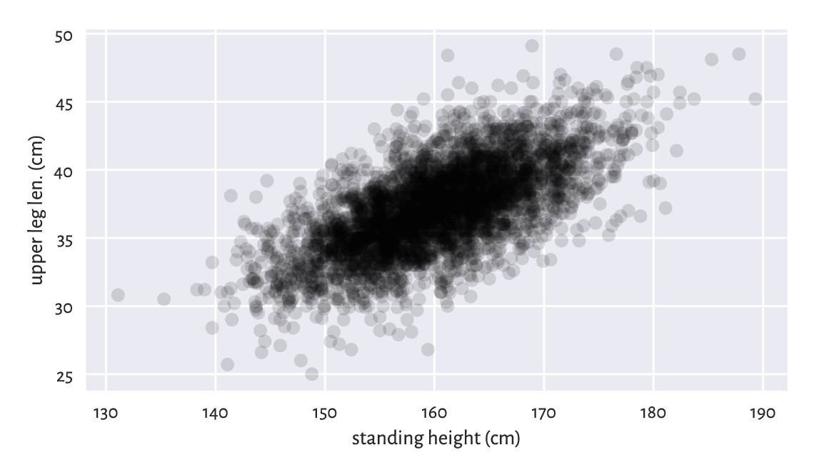
Figure 7.1 An example scatter plot.
Figure 7.1 depicts
upper leg length (the y-axis) vs (versus; against; as a function of)
standing height (the x-axis) in the form
of a point cloud with \((x, y)\) coordinates like
(body[i, 1], body[i, 3]) for all \(i=1,\dots,4221\).
Here are the exact coordinates of the point corresponding to the person of the smallest height:
body[np.argmin(body[:, 1]), [1, 3]]
## array([131.1,  30.8])
Locate it in Figure 7.1. Also, pinpoint the one with the greatest upper leg length:
body[np.argmax(body[:, 3]), [1, 3]]
## array([168.9,  49.1])
As the points are abundant, normally we cannot easily see
where most of them are located. As a simple remedy, we plotted the points
using a semi-transparent colour. This gave a kind of the points’ density
estimate. The colour specifier was of the form #rrggbbaa,
giving the intensity of the red, green, blue, and alpha (opaqueness)
channel in four series of two hexadecimal digits (between 00 = 0
and ff = 255).
Overall, the plot reveals that there is a general tendency for small heights and small upper leg lengths to occur frequently together. The taller the person, the longer her legs on average, and vice verse.
But there is some natural variability: for example, looking at people of height roughly equal to 160 cm, their upper leg length can be anywhere between 25 ad 50 cm (range), yet we expect the majority to lie somewhere between 35 and 40 cm. Chapter 9 will explore two measures of correlation that will enable us to quantify the degree (strength) of association between variable pairs.
7.4.2. 3D data and beyond
With more variables to visualise, we might be tempted to use a three-dimensional scatter plot like the one in Figure 7.2.
fig = plt.figure()
ax = fig.add_subplot(projection="3d", facecolor="#ffffff00")
ax.scatter(body[:, 1], body[:, 3], body[:, 0], color="#00000011")
ax.view_init(elev=30, azim=60, vertical_axis="y")
ax.set_xlabel(body_columns[1])
ax.set_ylabel(body_columns[3])
ax.set_zlabel(body_columns[0])
plt.show()
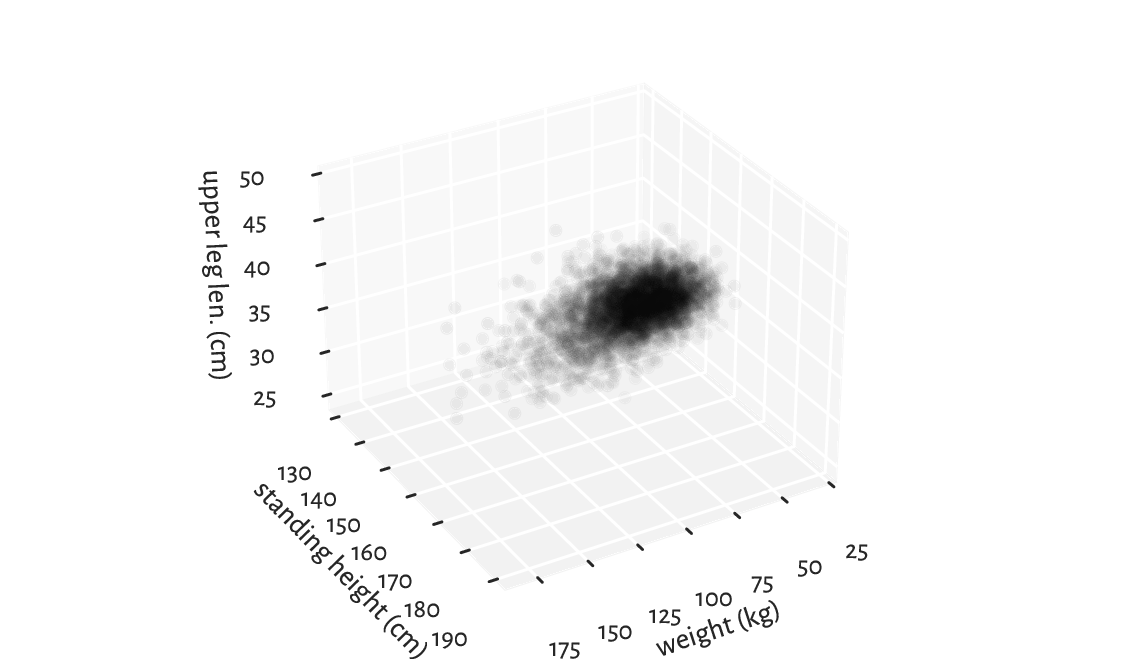
Figure 7.2 A three-dimensional scatter plot reveals almost nothing.
Infrequently will such a 3D plot provide us with readable results, though. We are projecting a three-dimensional reality onto a two-dimensional screen or a flat page. Some information must inherently be lost. What we see is relative to the position of the virtual camera and some angles can be more meaningful than others.
(*) Try finding an interesting elevation and azimuth angle by playing with the arguments passed to the mpl_toolkits.mplot3d.axes3d.Axes3D.view_init function. Also, depict arm circumference, hip circumference, and weight on a 3D plot.
Note
(*) We may have facilities for creating an interactive scatter plot (running the above from the Python’s console enables this), where the virtual camera can be freely repositioned with a mouse/touch pad. This can give some more insight into our data. Also, there are means of creating animated sequences, where we can fly over the data scene. Some people find it cool, others find it annoying, but the biggest problem therewith is that they cannot be included in printed material. If we are only targeting the display for the Web (this includes mobile devices), we can try some Python libraries that output HTML+CSS+JavaScript code which instructs the browser engine to create some more sophisticated interactive graphics, e.g., bokeh or plotly.
Instead of drawing a 3D plot, it might be better to play with a 2D scatter plot that uses different marker colours (or sometimes sizes: think of them as bubbles). Suitable colour maps can distinguish between low and high values of a third variable.
plt.scatter(
    body[:, 4],    # x
    body[:, 5],    # y
    c=body[:, 0],  # "z" - colours
    cmap=plt.colormaps.get_cmap("copper"),  # colour map
    alpha=0.5  # opaqueness level between 0 and 1
)
plt.xlabel(body_columns[4])
plt.ylabel(body_columns[5])
plt.axis("equal")
plt.rcParams["axes.grid"] = False
cbar = plt.colorbar()
plt.rcParams["axes.grid"] = True
cbar.set_label(body_columns[0])
plt.show()
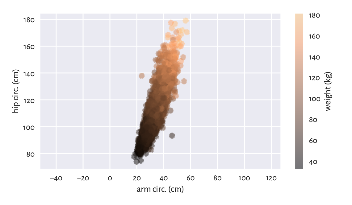
Figure 7.3 A two-dimensional scatter plot displaying three variables.
In Figure 7.3, we see some tendency for the weight to be greater as both the arm and the hip circumferences increase.
Play around with different colour palettes. However, be wary that every 1 in 12 men (8%) and 1 in 200 women (0.5%) have colour vision deficiencies, especially in the red-green or blue-yellow spectrum. For this reason, some diverging colour maps might be worse than others.
A piece of paper is two-dimensional: it only has height and width. By looking around, we also perceive the notion of depth. So far so good. But with more-dimensional data, well, suffice it to say that we are three-dimensional creatures and any attempts towards visualising them will simply not work, don’t even trip.
Luckily, it is where mathematics comes to our rescue. With some more knowledge and intuitions, and this book helps us develop them, it will be easy[5] to consider a generic \(m\)-dimensional space, and then assume that, say, \(m=7\) or \(42\). This is exactly why data science relies on automated methods for knowledge/pattern discovery. Thanks to them, we can identify, describe, and analyse the structures that might be present in the data, but cannot be experienced with our imperfect senses.
Note
Linear and nonlinear dimensionality reduction techniques can be applied to visualise some aspects of high-dimensional data in the form of 2D (or 3D) plots. In particular, the principal component analysis (PCA; Section 9.3) finds a potentially noteworthy angle from which we can try to look at the data.
7.4.3. Scatter plot matrix (pairs plot)
We can also try depicting all pairs of selected variables in the form of a scatter plot matrix.
def pairplot(X, labels, bins=21, alpha=0.1):
    """
    Draws a scatter plot matrix, given:
    * X - data matrix,
    * labels - list of column names
    """
    assert X.shape[1] == len(labels)

    k = X.shape[1]
    fig, axes = plt.subplots(nrows=k, ncols=k, sharex="col", sharey="row",
        figsize=(plt.rcParams["figure.figsize"][0], )*2)
    for i in range(k):
        for j in range(k):
            ax = axes[i, j]
            if i == j:  # diagonal
                ax.text(0.5, 0.5, labels[i], transform=ax.transAxes,
                    ha="center", va="center", size="x-small")
            else:
                ax.plot(X[:, j], X[:, i], ".", color="black", alpha=alpha)
And now:
which = [1, 0, 4, 5]
pairplot(body[:, which], body_columns[which])
plt.show()
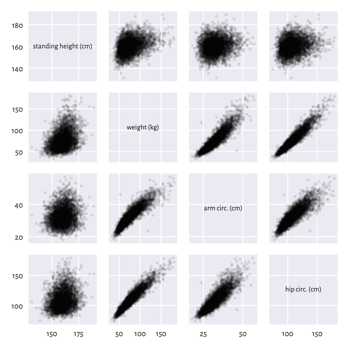
Figure 7.4 The scatter plot matrix for selected columns in the body dataset.
Plotting variables against themselves is rather silly (exercise: what would that be?). Therefore, on the main diagonal of Figure 7.4, we printed out the variable names.
A scatter plot matrix can be a valuable tool for identifying noteworthy combinations of columns in our datasets. We see that some pairs of variables are more “structured” than others, e.g., hip circumference and weight are more or less aligned on a straight line. This is why Chapter 9 will describe ways to model the possible relationships between the variables.
Create a pairs plot where weight, arm circumference, and hip circumference are on the log-scale.
(*) Call seaborn.pairplot to create a scatter plot matrix with histograms on the main diagonal, thanks to which you will be able to see how the marginal distributions are distributed. Note that the matrix must, unfortunately, be converted to a pandas data frame first.
(**) Modify our pairplot function so that it displays the histograms of the marginal distributions on the main diagonal.
7.5. Exercises
What is the difference between
[1, 2, 3], [[1, 2, 3]], and [[1], [2], [3]] in the context
of an array’s creation?
If A is a matrix with five rows and six columns,
what is the difference between A.reshape(6, 5) and A.T?
If A is a matrix with 5 rows and 6 columns,
what is the meaning of:
A.reshape(-1), A.reshape(3, -1),
A.reshape(-1, 3), A.reshape(-1, -1),
A.shape = (3, 10), and A.shape = (-1, 3)?
List some methods to add a new row or column to an existing matrix.
Give some ways to visualise three-dimensional data.
How can we set point opaqueness/transparency when drawing a scatter plot? When would we be interested in this?