8. Processing multidimensional data

This open-access textbook is, and will remain, freely available for everyone’s enjoyment (also in PDF; a paper copy can also be ordered). It is a non-profit project. Although available online, it is a whole course, and should be read from the beginning to the end. Refer to the Preface for general introductory remarks. Any bug/typo reports/fixes are appreciated. Make sure to check out Deep R Programming [36] too.

8.1. Extending vectorised operations to matrices

The vector operations from Chapter 5 are brilliant examples of the write less, do more principle in practice. Let’s see how are they extended to matrices.

8.1.1. Vectorised mathematical functions

Applying vectorised functions such as numpy.round, numpy.log, and numpy.exp returns an array of the same shape, with all elements transformed accordingly:

\[ f(\mathbf{X})= \left[ \begin{array}{cccc} f(x_{1,1}) & f(x_{1,2}) & \cdots & f(x_{1,m}) \\ f(x_{2,1}) & f(x_{2,2}) & \cdots & f(x_{2,m}) \\ \vdots & \vdots & \ddots & \vdots \\ f(x_{n,1}) & f(x_{n,2}) & \cdots & f(x_{n,m}) \\ \end{array} \right]. \]

A = np.array([
    [0.2, 0.6, 0.4, 0.4],
    [0.0, 0.2, 0.4, 0.7],
    [0.8, 0.8, 0.2, 0.1]
])  # example matrix

For instance, to take the square of every element, we can call:

np.square(A)
## array([[0.04, 0.36, 0.16, 0.16],
##        [0.  , 0.04, 0.16, 0.49],
##        [0.64, 0.64, 0.04, 0.01]])

8.1.2. Componentwise aggregation

Unidimensional aggregation functions (e.g., numpy.mean, numpy.quantile) can be applied to summarise:

• all data into a single number (axis=None, being the default),

• data in each column (axis=0), as well as

• data in each row (axis=1).

Here are the corresponding examples:

np.mean(A)
## 0.39999999999999997
np.mean(A, axis=0)
## array([0.33333333, 0.53333333, 0.33333333, 0.4       ])
np.mean(A, axis=1)
## array([0.4  , 0.325, 0.475])

Important

Let’s stress that axis=1 does not mean that we get the column means (even though columns constitute the second axis, and we count starting at 0). It denotes the axis along which the matrix is sliced. Sadly, even yours truly sometimes does not get it right.

Exercise 8.1

Given the nhanes_adult_female_bmx_2020 dataset, compute the mean, standard deviation, the minimum, and the maximum of each body measure.

We will get back to the topic of the aggregation of multidimensional data in Section 8.4.

8.1.3. Arithmetic, logical, and relational operations

Recall that for vectors, binary operators such as `+`, `*`, `==`, `<=`, and `&` as well as similar elementwise functions (e.g., numpy.minimum) can be applied if both inputs are of the same length. For example:

np.array([1, 10, 100, 1000]) * np.array([7, -6, 2, 8])  # elementwisely
## array([   7,  -60,  200, 8000])

Alternatively, one input can be a scalar:

np.array([1, 10, 100, 1000]) * -3
## array([   -3,   -30,  -300, -3000])

More generally, a set of rules referred to in the numpy manual as broadcasting describes how this package handles arrays of different shapes.

Important

Generally, for two matrices, their column/row counts must match or be equal to 1. Also, if one operand is a one-dimensional array, it will be promoted to a row vector.

Let’s explore all the possible scenarios.

8.1.3.1. Matrix vs scalar

If one operand is a scalar, then it is going to be propagated over all matrix elements. For example:

(-1)*A
## array([[-0.2, -0.6, -0.4, -0.4],
##        [-0. , -0.2, -0.4, -0.7],
##        [-0.8, -0.8, -0.2, -0.1]])

It changed the sign of every element, which is, mathematically, an instance of multiplying a matrix \(\mathbf{X}\) by a scalar \(c\):

\[ c\mathbf{X}= \left[ \begin{array}{cccc} cx_{1,1} & cx_{1,2} & \cdots & cx_{1,m} \\ cx_{2,1} & cx_{2,2} & \cdots & cx_{2,m} \\ \vdots & \vdots & \ddots & \vdots \\ cx_{n,1} & cx_{n,2} & \cdots & cx_{n,m} \\ \end{array} \right]. \]

Furthermore, we can take the square[1] of each element:

A**2
## array([[0.04, 0.36, 0.16, 0.16],
##        [0.  , 0.04, 0.16, 0.49],
##        [0.64, 0.64, 0.04, 0.01]])

or compare each element to 0.25.

A >= 0.25
## array([[False,  True,  True,  True],
##        [False, False,  True,  True],
##        [ True,  True, False, False]])

8.1.3.2. Matrix vs matrix

For two matrices of identical sizes, we act on the corresponding elements:

B = np.tri(A.shape[0], A.shape[1])  # just an example
B  # a lower triangular 0-1 matrix
## array([[1., 0., 0., 0.],
##        [1., 1., 0., 0.],
##        [1., 1., 1., 0.]])

And now:

A * B
## array([[0.2, 0. , 0. , 0. ],
##        [0. , 0.2, 0. , 0. ],
##        [0.8, 0.8, 0.2, 0. ]])

multiplies each \(a_{i,j}\) by the corresponding \(b_{i,j}\).

This behaviour extends upon the idea from algebra that given \(\mathbf{A}\) and \(\mathbf{B}\) with \(n\) rows and \(m\) columns each, the result of \(+\) is:

\[ \mathbf{A} + \mathbf{B}= \left[ \begin{array}{cccc} a_{1,1}+b_{1,1} & a_{1,2}+b_{1,2} & \cdots & a_{1,m}+b_{1,m} \\ a_{2,1}+b_{2,1} & a_{2,2}+b_{2,2} & \cdots & a_{2,m}+b_{2,m} \\ \vdots & \vdots & \ddots & \vdots \\ a_{n,1}+b_{n,1} & a_{n,2}+b_{n,2} & \cdots & a_{n,m}+b_{n,m} \\ \end{array} \right]. \]

Thanks to the matrix-matrix and matrix-scalar operations, we can perform various tests on a per-element basis, e.g.,

(A >= 0.25) & (A <= 0.75)  # logical matrix & logical matrix
## array([[False,  True,  True,  True],
##        [False, False,  True,  True],
##        [False, False, False, False]])

Example 8.2

(*) Figure 8.1 depicts a (filled) contour plot of Himmelblau’s function, \(f(x,y)=(x^{2}+y-11)^{2}+(x+y^{2}-7)^{2}\), for \(x\in[-5, 5]\) and \(y\in[-4, 4]\). To draw it, we probe 250 points from these two intervals, and call numpy.meshgrid to generate two matrices, both of shape 250 by 250, giving the x- and y-coordinates of all the points on the corresponding two-dimensional grid. Thanks to this, we are able to use vectorised mathematical operations to compute the values of \(f\) thereon.

x = np.linspace(-5, 5, 250)
y = np.linspace(-4, 4, 250)
xg, yg = np.meshgrid(x, y)
z = (xg**2 + yg - 11)**2 + (xg + yg**2 - 7)**2
plt.contourf(x, y, z, levels=20)
CS = plt.contour(x, y, z, levels=[1, 5, 10, 20, 50, 100, 150, 200, 250])
plt.clabel(CS, colors="black")
plt.show()

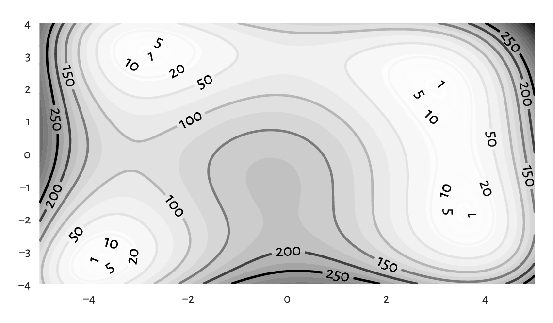
Figure 8.1 An example filled contour plot with additional labelled contour lines.

To understand the result generated by numpy.meshgrid, let’s inspect its output for a smaller number of probe points:

x = np.linspace(-5, 5, 3)
y = np.linspace(-4, 4, 5)
xg, yg = np.meshgrid(x, y)
xg
## array([[-5.,  0.,  5.],
##        [-5.,  0.,  5.],
##        [-5.,  0.,  5.],
##        [-5.,  0.,  5.],
##        [-5.,  0.,  5.]])

Here, each column consists of the same values.

yg
## array([[-4., -4., -4.],
##        [-2., -2., -2.],
##        [ 0.,  0.,  0.],
##        [ 2.,  2.,  2.],
##        [ 4.,  4.,  4.]])

In this case, each row is constant. Therefore, calling:

(xg**2 + yg - 11)**2 + (xg + yg**2 - 7)**2
## array([[116., 306., 296.],
##        [208., 178., 148.],
##        [340., 170., 200.],
##        [320.,  90., 260.],
##        [340., 130., 520.]])

gives a matrix \(\mathbf{Z}\) such that \(z_{i,j}\) is generated by considering the \(i\)-th element in y and the \(j\)-th item in x, which is exactly what we desired. We will provide an alternative implementation in Example 8.5.

8.1.3.3. Matrix vs any vector

An n×m matrix can also be combined with an n×1 column vector:

A * np.array([1, 10, 100]).reshape(-1, 1)
## array([[ 0.2,  0.6,  0.4,  0.4],
##        [ 0. ,  2. ,  4. ,  7. ],
##        [80. , 80. , 20. , 10. ]])

It propagated the column vector over all columns (left to right). Similarly, combining a matrix with a 1×m row vector recycles the latter over all rows (top to bottom).

A + np.array([1, 2, 3, 4]).reshape(1, -1)
## array([[1.2, 2.6, 3.4, 4.4],
##        [1. , 2.2, 3.4, 4.7],
##        [1.8, 2.8, 3.2, 4.1]])

If one operand is a one-dimensional array or a list of length \(m\), it will be treated as a row vector. For example, here is an instance of centring of each column:

np.round(A - np.mean(A, axis=0), 3)  # matrix - vector
## array([[-0.133,  0.067,  0.067, -0.   ],
##        [-0.333, -0.333,  0.067,  0.3  ],
##        [ 0.467,  0.267, -0.133, -0.3  ]])

An explicit .reshape(1, -1) was not necessary.

Mathematically, although it is not necessarily a standard notation, we will allow adding and subtracting row vectors from matrices of compatible sizes:

\[ \mathbf{X}+\mathbf{t}= \mathbf{X}+[ t_1\ t_2\ \cdots\ t_m ]= \left[ \begin{array}{cccc} x_{1,1} + t_1 & x_{1,2} + t_2 & \dots & x_{1,m} + t_m \\ x_{2,1} + t_1 & x_{2,2} + t_2 & \dots & x_{2,m} + t_m \\ \vdots & \vdots & \ddots & \vdots \\ x_{n,1} + t_1 & x_{n,2} + t_2 & \dots & x_{n,m} + t_m \\ \end{array} \right]. \]

This corresponds to shifting (translating) every row in the matrix.

Exercise 8.3

In the nhanes_adult_female_bmx_2020 dataset, standardise, normalise, and min-max scale every column (compare Section 5.3.2). A single line of code will suffice in each case.

8.1.3.4. Row vector vs column vector (*)

A row vector combined with a column vector results in an operation’s being performed on each combination of all pairs of elements in the two arrays (i.e., the cross-product; not just the corresponding pairs).

np.arange(1, 8).reshape(1, -1) * np.array([1, 10, 100]).reshape(-1, 1)
## array([[  1,   2,   3,   4,   5,   6,   7],
##        [ 10,  20,  30,  40,  50,  60,  70],
##        [100, 200, 300, 400, 500, 600, 700]])

Exercise 8.4

Check out that numpy.nonzero relies on similar shape broadcasting rules as the binary operators we discussed here, but not with respect to all three arguments.

Example 8.5

(*) Himmelblau’s function in Example 8.2 is defined by means of arithmetic operators only, and they all rely on the kind of shape broadcasting that we discuss in this section. Consequently, calling numpy.meshgrid to evaluate \(f\) on a point grid was not really necessary:

x = np.linspace(-5, 5, 3)
y = np.linspace(-4, 4, 5)
xg = x.reshape(1, -1)
yg = y.reshape(-1, 1)
(xg**2 + yg - 11)**2 + (xg + yg**2 - 7)**2
## array([[116., 306., 296.],
##        [208., 178., 148.],
##        [340., 170., 200.],
##        [320.,  90., 260.],
##        [340., 130., 520.]])

See also the sparse parameter in numpy.meshgrid, and Section 12.3.1 where this function turns out useful after all.

8.1.4. Other row and column transforms (*)

Some functions discussed in the previous part of this course are equipped with the axis argument, which supports processing each row or column independently. For example, to compute the ranks of elements in each column, we can call:

scipy.stats.rankdata(A, axis=0)  # columnwisely (along the rows)
## array([[2. , 2. , 2.5, 2. ],
##        [1. , 1. , 2.5, 3. ],
##        [3. , 3. , 1. , 1. ]])

Some functions have the default argument axis=-1 meaning that they are applied along the last[2] axis (i.e., columns in the matrix case):

np.diff(A)  # means axis=1 in this context (along the columns)
## array([[ 0.4, -0.2,  0. ],
##        [ 0.2,  0.2,  0.3],
##        [ 0. , -0.6, -0.1]])

Compare the foregoing to the iterated differences in each column separately (along the rows):

np.diff(A, axis=0)
## array([[-0.2, -0.4,  0. ,  0.3],
##        [ 0.8,  0.6, -0.2, -0.6]])

If a vectorised function in not equipped with the axis argument, we can propagate it over all the rows or columns by calling numpy.apply_along_axis. For instance, here is another (did you solve Exercise 8.3?) way to compute the z-scores in each matrix column:

def standardise(x):
    return (x-np.mean(x))/np.std(x)

np.round(np.apply_along_axis(standardise, 0, A), 2)  # round for readability
## array([[-0.39,  0.27,  0.71, -0.  ],
##        [-0.98, -1.34,  0.71,  1.22],
##        [ 1.37,  1.07, -1.41, -1.22]])

But, of course, we prefer (x-np.mean(x, axis=0))/np.std(x, axis=0).

Note

(*) Matrices are iterable (in the sense of Section 3.4), but in an interesting way. Namely, an iterator traverses through each row in a matrix. Writing:

r1, r2, r3 = A  # A has three rows

creates three variables, each representing a separate row in A, the second of which is:

r2
## array([0. , 0.2, 0.4, 0.7])

8.2. Indexing matrices

Recall that for unidimensional arrays, we have four possible indexer choices (i.e., when performing filtering like x[i]):

• scalar (extracts a single element),

• slice (selects a regular subsequence, e.g., every second element or the first six items; returns a view of existing data: it does not make an independent copy of the subsetted elements),

• integer vector (selects the elements at given indexes),

• logical vector (selects the elements that correspond to True in the indexer).

Matrices are two-dimensional arrays. Subsetting thus requires two indexes. By writing A[i, j], we select rows given by i and columns given by j. Both i and j can be one of the four aforementioned types, so we have at ten different cases to consider (skipping the symmetric ones).

Important

Generally:

• each scalar index reduces the dimensionality of the subsetted object by 1;

• slice-slice and slice-scalar indexing returns a view of the existing array, so we need to be careful when modifying the resulting object;

• usually, indexing returns a submatrix (subblock), which is a combination of elements at given rows and columns;

• indexing with two integer or logical vectors is performed elementwisely, and should be avoided if find the rules of shape broadcasting too complicated.

8.2.1. Slice-based indexing

Our favourite example matrix again:

A = np.array([
    [0.2, 0.6, 0.4, 0.4],
    [0.0, 0.2, 0.4, 0.7],
    [0.8, 0.8, 0.2, 0.1]
])

Indexing based on two slices selects a submatrix:

A[::2, 3:]  # every second row, skip the first three columns
## array([[0.4],
##        [0.1]])

An empty slice selects all elements on the corresponding axis:

A[:, ::-1]  # all rows, reversed columns
## array([[0.4, 0.4, 0.6, 0.2],
##        [0.7, 0.4, 0.2, 0. ],
##        [0.1, 0.2, 0.8, 0.8]])

Let’s stress that the result is always in the form of a matrix.

8.2.2. Scalar-based indexing

Indexing by a scalar selects a given row or column, reducing the dimensionality of the output object:

A[:, 3]  # one scalar: from two to one dimensions
## array([0.4, 0.7, 0.1])

It selected the fourth column and gave a flat vector (we can always use the reshape method to convert the resulting object back to a matrix). Furthermore:

A[0, -1]  # two scalars: from two to zero dimensions
## 0.4

It yielded the element (scalar) in the first row and the last column.

8.2.3. Mixed logical/integer vector and scalar/slice indexers

A logical and integer vector-like object can also be employed for element selection. If the other indexer is a slice or a scalar, the result is quite predictable. For instance:

A[ [0, -1, 0], ::-1 ]
## array([[0.4, 0.4, 0.6, 0.2],
##        [0.1, 0.2, 0.8, 0.8],
##        [0.4, 0.4, 0.6, 0.2]])

It selected the first, the last, and the first row again. Then, it reversed the order of columns.

A[ A[:, 0] > 0.1, : ]
## array([[0.2, 0.6, 0.4, 0.4],
##        [0.8, 0.8, 0.2, 0.1]])

It chose the rows from A where the values in the first column of A are greater than 0.1.

A[np.mean(A, axis=1) > 0.35, : ]
## array([[0.2, 0.6, 0.4, 0.4],
##        [0.8, 0.8, 0.2, 0.1]])

It fetched the rows whose mean is greater than 0.35.

A[np.argsort(A[:, 0]), : ]
## array([[0. , 0.2, 0.4, 0.7],
##        [0.2, 0.6, 0.4, 0.4],
##        [0.8, 0.8, 0.2, 0.1]])

It ordered the matrix with respect to the values in the first column (all rows permuted in the same way, together).

Exercise 8.6

In the nhanes_adult_female_bmx_2020 dataset, select all the participants whose heights are within their mean ± 2 standard deviations.

8.2.4. Two vectors as indexers (*)

Indexing based on two logical or integer vectors is a tad more horrible, as in this case not only some form of shape broadcasting comes into play but also all the headache-inducing exceptions listed in the perhaps not the most clearly written Advanced Indexing section of the numpy manual. Cheer up, though: Section 10.5 points out that indexing in pandas is even more troublesome.

For the sake of our maintaining sanity, in practice, it is best to be extra careful when using two vector indexers and stick only to the scenarios discussed beneath. First, with two flat integer indexers, we pick elementwisely:

A[ [0, -1, 0, 2, 0], [1, 2, 0, 2, 1] ]
## array([0.6, 0.2, 0.2, 0.2, 0.6])

It yielded A[0, 1], A[-1, 2], A[0, 0], A[2, 2], and A[0, 1].

Second, to select a submatrix (a subblock) using integer indexes, it is best to make sure that the first indexer is a column vector, and the second one is a row vector (or some objects like these, e.g., compatible lists of lists).

A[ [[0], [-1]], [[1, 3]] ]  # column vector-like list, row vector-like list
## array([[0.6, 0.4],
##        [0.8, 0.1]])

Third, if indexing involves logical vectors, it is best to convert them to integer ones first (e.g., by calling numpy.flatnonzero).

A[ np.flatnonzero(np.mean(A, axis=1) > 0.35).reshape(-1, 1), [[0, 2, 3, 0]] ]
## array([[0.2, 0.4, 0.4, 0.2],
##        [0.8, 0.2, 0.1, 0.8]])

The necessary reshaping can be outsourced to numpy.ix_ function:

A[ np.ix_( np.mean(A, axis=1) > 0.35, [0, 2, 3, 0] ) ]  # np.ix_(rows, cols)
## array([[0.2, 0.4, 0.4, 0.2],
##        [0.8, 0.2, 0.1, 0.8]])

Alternatively, we can always apply indexing twice:

A[np.mean(A, axis=1) > 0.45, :][:, [0, 2, 3, 0]]
## array([[0.8, 0.2, 0.1, 0.8]])

This is only a mild inconvenience. We will be forced to apply such double indexing anyway in pandas whenever selecting rows by position and columns by name is required; see Section 10.5.

Note

(*) Interestingly, we can also index a vector using an integer matrix. This is like subsetting using a list of integer indexes, but the output’s shape matches that of the indexer:

u = np.array(["a", "b", "c"])
V = np.array([ [0, 1], [1, 0], [2, 1] ])
u[V]  # like u[V.ravel()].reshape(V.shape)
## array([['a', 'b'],
##        ['b', 'a'],
##        ['c', 'b']], dtype='<U1')

8.2.5. Views of existing arrays (*)

Only the indexing involving two slices or a slice and a scalar returns a view on an existing array. For example:

B = A[:, ::2]
B
## array([[0.2, 0.4],
##        [0. , 0.4],
##        [0.8, 0.2]])

Now B and A share memory. By modifying B in place, e.g.:

B *= -1

the changes will be visible in A as well:

A
## array([[-0.2,  0.6, -0.4,  0.4],
##        [-0. ,  0.2, -0.4,  0.7],
##        [-0.8,  0.8, -0.2,  0.1]])

This is time and memory efficient, but might lead to some unexpected results if we are being rather absent-minded. The readers have been warned.

In all other cases, we get a copy of the subsetted array.

8.2.6. Adding and modifying rows and columns

With slice- and scalar-based indexers, rows, columns, or individual elements can be replaced by new content in a natural way:

A[:, 0] = A[:, 0]**2

With numpy arrays, however, new rows or columns cannot be added via the index operator. Instead, the whole array needs to be created from scratch using, e.g., one of the functions discussed in Section 7.1.4. For example:

A = np.column_stack((A, np.sqrt(A[:, 0])))
A
## array([[ 0.04,  0.6 , -0.4 ,  0.4 ,  0.2 ],
##        [ 0.  ,  0.2 , -0.4 ,  0.7 ,  0.  ],
##        [ 0.64,  0.8 , -0.2 ,  0.1 ,  0.8 ]])

8.3. Matrix multiplication, dot products, and Euclidean norm (*)

Matrix algebra is at the core of all the methods used in data analysis with the matrix multiplication being often the most crucial operation (e.g., [22, 42]). Given \(\mathbf{A}\in\mathbb{R}^{n\times p}\) and \(\mathbf{B}\in\mathbb{R}^{p\times m}\), their multiply is a matrix \(\mathbf{C}=\mathbf{A}\mathbf{B}\in\mathbb{R}^{n\times m}\) such that \(c_{i,j}\) is the sum of the \(i\)-th row in \(\mathbf{A}\) and the \(j\)-th column in \(\mathbf{B}\) multiplied elementwisely:

\[ c_{i,j} = a_{i, 1} b_{1, j} + a_{i, 2} b_{2, j} + \dots + a_{i, p} b_{p, j} = \sum_{k=1}^p a_{i,k} b_{k, j}, \]

for \(i=1,\dots,n\) and \(j=1,\dots,m\). For example:

A = np.array([
    [1, 0, 1],
    [2, 2, 1],
    [3, 2, 0],
    [1, 2, 3],
    [0, 0, 1],
])
B = np.array([
    [1, 0, 0, 0],
    [0, 4, 1, 3],
    [2, 0, 3, 1],
])

And now:

C = A @ B  # or: A.dot(B)
C
## array([[ 3,  0,  3,  1],
##        [ 4,  8,  5,  7],
##        [ 3,  8,  2,  6],
##        [ 7,  8, 11,  9],
##        [ 2,  0,  3,  1]])

Mathematically, we can denote it by:

\[ \left[ \begin{array}{ccc} 1 & 0 & 1 \\ 2 & 2 & 1 \\ 3 & 2 & 0 \\ \mathbf{1} & \mathbf{2} & \mathbf{3} \\ 0 & 0 & 1 \\ \end{array} \right] \, \left[ \begin{array}{cccc} 1 & 0 & \mathbf{0} & 0 \\ 0 & 4 & \mathbf{1} & 3 \\ 2 & 0 & \mathbf{3} & 1 \\ \end{array} \right] = \left[ \begin{array}{cccc} 3 & 0 & 3 & 1 \\ 4 & 8 & 5 & 7 \\ 3 & 8 & 2 & 6 \\ 7 & 8 & \mathbf{11} & 9 \\ 2 & 0 & 3 & 1 \\ \end{array} \right]. \]

For example, the element in the fourth row and the third column, \(c_{4,3}\) takes the fourth row in the left matrix \(\mathbf{a}_{4,\cdot}=[1\ 2\ 3]\) and the third column in the right matrix \(\mathbf{b}_{\cdot,3}=[0\ 1\ 3]^T\) (emphasised with bold), multiplies the corresponding elements, and computes their sum, i.e., \(c_{4,3}=1\cdot 0 + 2\cdot 1 + 3\cdot 3 = 11\).

Important

Matrix multiplication can only be performed on two matrices of compatible sizes: the number of columns in the left matrix must match the number of rows in the right operand.

Another example:

A = np.array([
    [1, 2],
    [3, 4]
])
I = np.array([  # np.eye(2)
    [1, 0],
    [0, 1]
])
A @ I  # or A.dot(I)
## array([[1, 2],
##        [3, 4]])

We matrix-multiplied \(\mathbf{A}\) by the identity matrix \(\mathbf{I}\), which is the neutral element of the said operation. This is why the result is identical to \(\mathbf{A}\).

Important

In most textbooks, just like in this one, \(\mathbf{A}\mathbf{B}\) always denotes the matrix multiplication. This is a very different operation from the elementwise multiplication.

Compare the above to:

A * I  # elementwise multiplication (the Hadamard product)
## array([[1, 0],
##        [0, 4]])

Exercise 8.7

(*) Show that \((\mathbf{A}\mathbf{B})^T=\mathbf{B}^T \mathbf{A}^T\). Also notice that, typically, matrix multiplication is not commutative, i.e., \(\mathbf{A}\mathbf{B}\neq\mathbf{B}\mathbf{A}\).

Note

By definition, matrix multiplication is convenient for denoting sums of products of corresponding elements in many pairs of vectors, which we refer to as dot products. More formally, given two vectors \(\boldsymbol{x}, \boldsymbol{y} \in \mathbb{R}^p\), their dot (or scalar) product is:

\[ \boldsymbol{x} \cdot \boldsymbol{y} = \sum_{i=1}^p x_i y_i. \]

In matrix multiplication terms, if \(\mathbf{x}\) is a row vector and \(\mathbf{y}^T\) is a column vector, then the above can be written as \(\mathbf{x} \mathbf{y}^T\). The result is a single number.

In particular, the dot product of a vector and itself:

\[ \boldsymbol{x} \cdot \boldsymbol{x} = \sum_{i=1}^p x_i^2, \]

is the square of the Euclidean norm of \(\boldsymbol{x}\) (simply the sum of squares), which is used to measure the magnitude of a vector (Section 5.3.2.3):

\[ \|\boldsymbol{x}\| = \sqrt{\sum_{i=1}^p x_i^2} =\sqrt{\boldsymbol{x} \cdot \boldsymbol{x}} =\sqrt{\mathbf{x} \mathbf{x}^T}. \]

It is worth pointing out that the Euclidean norm fulfils (amongst others) the condition that \(\|\boldsymbol{x}\|=0\) if and only if \(\boldsymbol{x}=\mathbf{0}=(0,0,\dots,0)\). The same naturally holds for its square.

Exercise 8.8

Show that \(\mathbf{A}^T \mathbf{A}\) gives the matrix that consists of the dot products of all the pairs of columns in \(\mathbf{A}\) and \(\mathbf{A} \mathbf{A}^T\) stores the dot products of all the pairs of rows.

Section 9.3.2 will note that matrix multiplication can be used as a way to express certain geometrical transformations of points in a dataset, e.g., scaling and rotating. Also, Section 9.3.3 briefly discusses the concept of the inverse of a matrix. Furthermore, Section 9.3.4 introduces its singular value decomposition.

8.4. Pairwise distances and related methods (*)

Many data analysis methods rely on the notion of distances, which quantify the extent to which two points (e.g., two rows in a matrix) differ from each other. Here, we will be dealing with the most natural[3] distance called the Euclidean metric. We know it from school, where we measured it using a ruler.

8.4.1. Euclidean metric (*)

Given two points in \(\mathbb{R}^m\), \(\boldsymbol{u}=(u_1,\dots,u_m)\) and \(\boldsymbol{v}=(v_1,\dots,v_m)\), the Euclidean metric is defined in terms of the corresponding Euclidean norm:

\[ \|\boldsymbol{u} - \boldsymbol{v}\| = \sqrt{ (u_1-v_1)^2 + (u_2-v_2)^2 + \dots + (u_m-v_m)^2 } = \sqrt{ \sum_{i=1}^m (u_i-v_i)^2 }, \]

i.e., the square root of the sum of squared differences between the corresponding coordinates.

In particular, for unidimensional data (\(m=1\)), we have \(\|\boldsymbol{u}-\boldsymbol{v}\|=|u_1-v_1|\), i.e., the absolute value of the difference.

Important

Given two vectors of equal lengths \(\boldsymbol{x},\boldsymbol{y}\in\mathbb{R}^m\), the dot product of their difference:

\[ (\boldsymbol{x}-\boldsymbol{y})\cdot (\boldsymbol{x}-\boldsymbol{y}) = (\mathbf{x}-\mathbf{y}) (\mathbf{x}-\mathbf{y})^T = \sum_{i=1}^{m} (x_i-y_i)^2, \]

is nothing else than the square of the Euclidean distance between them.

Exercise 8.9

Consider the following matrix \(\mathbf{X}\in\mathbb{R}^{4\times 2}\):

\[ \mathbf{X} = \left[\begin{array}{cc} 0 & 0 \\ 1 & 0 \\ -3/2 & 1 \\ 1 & 1 \\ \end{array}\right]. \]

Calculate (by hand): \(\|\mathbf{x}_{1,\cdot} - \mathbf{x}_{2,\cdot}\|\), \(\|\mathbf{x}_{1,\cdot} - \mathbf{x}_{3,\cdot}\|\), \(\|\mathbf{x}_{1,\cdot} - \mathbf{x}_{4,\cdot}\|\), \(\|\mathbf{x}_{2,\cdot} - \mathbf{x}_{4,\cdot}\|\), \(\|\mathbf{x}_{2,\cdot} - \mathbf{x}_{3,\cdot}\|\), \(\|\mathbf{x}_{1,\cdot} - \mathbf{x}_{1,\cdot}\|\), and \(\|\mathbf{x}_{2,\cdot} - \mathbf{x}_{1,\cdot}\|\).

scipy.spatial.distance.cdist computes the distances between all the possible pairs of rows in two matrices \(\mathbf{X}\in\mathbb{R}^{n\times m}\) and \(\mathbf{Y}\in\mathbb{R}^{k\times m}\). We need to be careful, though. It brings about a distance matrix of size \(n\times k\), which can become large. For instance, for \(n=k=100 000\), we need roughly 80 GB of RAM to store it.

Here are the distances between all the pairs of points in the same dataset.

X = np.array([
    [0,    0],
    [1,    0],
    [-1.5, 1],
    [1,    1]
])
import scipy.spatial.distance
D = scipy.spatial.distance.cdist(X, X)
D
## array([[0.        , 1.        , 1.80277564, 1.41421356],
##        [1.        , 0.        , 2.6925824 , 1.        ],
##        [1.80277564, 2.6925824 , 0.        , 2.5       ],
##        [1.41421356, 1.        , 2.5       , 0.        ]])

Hence, \(d_{i,j}=\|\mathbf{x}_{i,\cdot}-\mathbf{x}_{j,\cdot}\|\). That we have zeros on the diagonal is due to the fact that \(\|\boldsymbol{u} - \boldsymbol{v}\|= 0\) if and only if \(\boldsymbol{u} = \boldsymbol{v}\). Furthermore, \(\|\boldsymbol{u} - \boldsymbol{v}\|=\|\boldsymbol{v} - \boldsymbol{u}\|\), which implies the symmetry of \(\mathbf{D}\), i.e., we have \(\mathbf{D}^T=\mathbf{D}\).

Figure 8.2 illustrates the six non-trivial pairwise distances. In the left subplot, our perception of distance is disturbed because the aspect ratio (the ratio between the range of the x-axis to the range of the y-axis) is not 1:1. To be able to assess spatial relationships, it is thus very important to call matplotlib.pyplot.axis("equal").

for s in range(2):
    plt.subplot(1, 2, s+1)
    if s == 1: plt.axis("equal")  # right subplot
    plt.plot(X[:, 0], X[:, 1], "ko")
    for i in range(X.shape[0]-1):
        for j in range(i+1, X.shape[0]):
            plt.plot(X[[i,j], 0], X[[i,j], 1], "k-", alpha=0.2)
            plt.text(
                np.mean(X[[i,j], 0]),
                np.mean(X[[i,j], 1]),
                np.round(D[i, j], 2)
            )
plt.show()

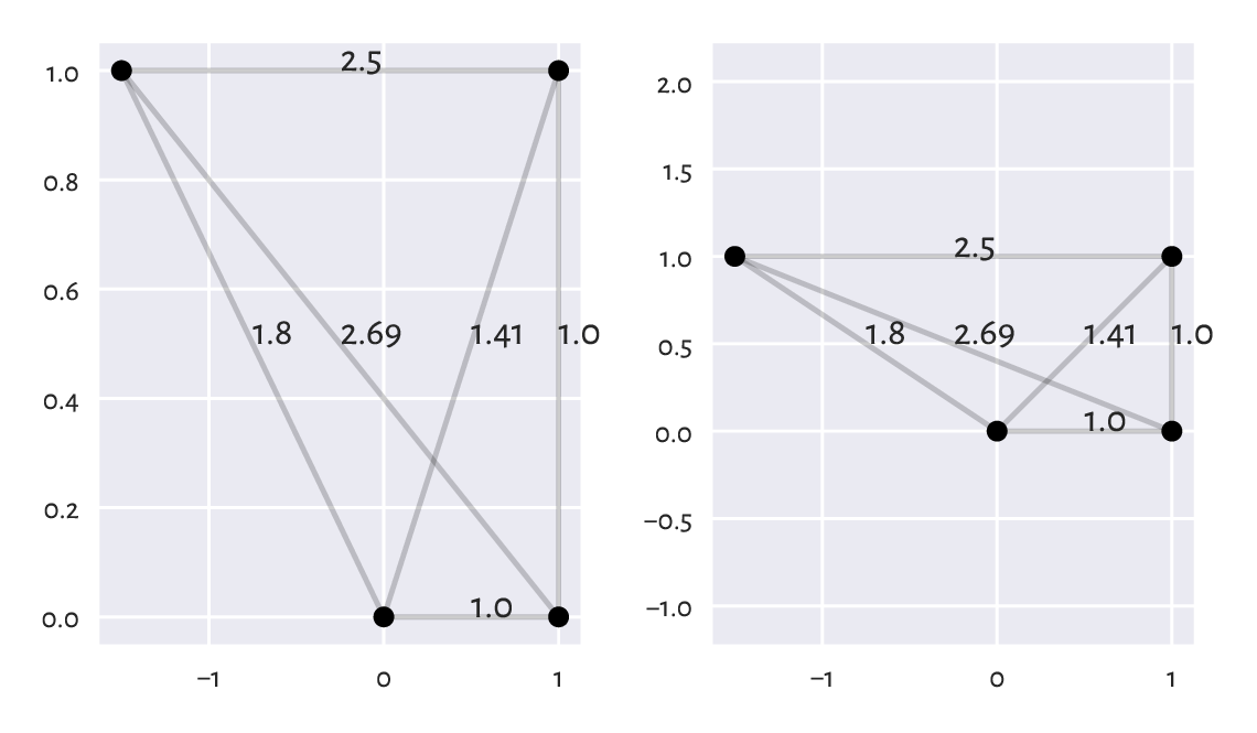
Figure 8.2 Distances between four example points. In the left plot, their perception is disturbed because the aspect ratio is not 1:1.

Exercise 8.10

(*) Each metric also enjoys the triangle inequality: \(\|\boldsymbol{u} - \boldsymbol{v}\| \le \|\boldsymbol{u} - \boldsymbol{w}\| + \|\boldsymbol{w} - \boldsymbol{v}\|\) for all \(\boldsymbol{u}, \boldsymbol{v}, \boldsymbol{w}\). Verify that this property holds by studying each triple of points in an example distance matrix.

Important

A few popular data science techniques rely on pairwise distances, e.g.:

• multidimensional data aggregation (undermentioned),

• \(k\)-means clustering (Section 12.4),

• \(k\)-nearest neighbour regression (Section 9.2.1) and classification (Section 12.3.1),

• missing value imputation (Section 15.1),

• density estimation (which we can use outlier detection, see Section 15.4).

They assume that data have been appropriately preprocessed; compare, e.g., [2]. In particular, matrix columns should be on the same scale (e.g., standardised) as otherwise computing sums of their squared differences might not make sense at all.

8.4.2. Centroids (*)

So far we have been only discussing ways to aggregate unidimensional data, e.g., each matrix column separately. Some of the introduced summaries can be generalised to the multidimensional case.

For instance, the arithmetic mean of a vector \((x_1,\dots,x_n)\) is a point \(c\) that minimises the sum of the squared unidimensional distances between itself and all the \(x_i\)s, i.e., the minimiser of \(\sum_{i=1}^n \|x_i-c\|^2=\sum_{i=1}^n (x_i-c)^2\). More generally, we can define the centroid of a dataset \(\mathbf{X}\in\mathbb{R}^{n\times m}\) as the point \(\boldsymbol{c}\in\mathbb{R}^m\) to which the overall squared distance is the smallest:

\[ \text{minimise}\ \sum_{i=1}^n \| \mathbf{x}_{i,\cdot}-\boldsymbol{c}\|^2 \qquad\text{w.r.t. }\boldsymbol{c}. \]

Its solution is:

\[ \boldsymbol{c} = \frac{1}{n}\left( \mathbf{x}_{1, \cdot}+\mathbf{x}_{2, \cdot}+\dots+\mathbf{x}_{n, \cdot} \right) = \frac{1}{n} \sum_{i=1}^n \mathbf{x}_{i, \cdot}, \]

which is the componentwise (columnwise) arithmetic mean. In other words, its \(j\)-th component is given by:

\[ c_j = \frac{1}{n} \sum_{i=1}^n x_{i, j}. \]

For example, the centroid of the dataset depicted in Figure 8.2 is:

c = np.mean(X, axis=0)
c
## array([0.125, 0.5  ])

Centroids are the basis for the \(k\)-means clustering method that we discuss in Section 12.4.

8.4.3. Multidimensional dispersion and other aggregates (**)

Furthermore, as a measure of multidimensional dispersion, we can consider the natural generalisation of the standard deviation:

\[ s= \sqrt{ \frac{1}{n} \sum_{i=1}^n \| \mathbf{x}_{i,\cdot}-\boldsymbol{c}\|^2 }, \]

being the square root of the average squared distance to the centroid. Notice that \(s\) is a single number.

np.sqrt(np.mean(scipy.spatial.distance.cdist(X, c.reshape(1, -1))**2))
## 1.1388041973930374

Note

(**) Generalising other aggregation functions is not a trivial task because, amongst others, there is no natural linear ordering relation in the multidimensional space (see, e.g., [78]). For instance, any point on the convex hull of a dataset could serve as an analogue of the minimal and maximal observation.

Furthermore, the componentwise median does not behave nicely (it may, for example, fall outside the convex hull). Instead, we usually consider a different generalisation of the median: the point \(\boldsymbol{m}\) which minimises the sum of distances (not squared), \(\sum_{i=1}^n \| \mathbf{x}_{i,\cdot}-\boldsymbol{m}\|\). Even though it does not have an analytic solution, it can be determined algorithmically.

Note

(**) A bag plot [84] is one of the possible multidimensional generalisations of the box-and-whisker plot. Unfortunately, its use is not popular amongst practitioners.

8.4.4. Fixed-radius and k-nearest neighbour search (**)

Several data analysis techniques rely on aggregating information about what is happening in the local neighbourhoods of given points. Let \(\mathbf{X}\in\mathbb{R}^{n\times m}\) be a dataset and \(\boldsymbol{x}'\in\mathbb{R}^m\) be some point, not necessarily from \(\mathbf{X}\). We have two options:

• fixed-radius search: for some radius \(r>0\), we seek the indexes of all the points in \(\mathbf{X}\) whose distance to \(\boldsymbol{x}'\) is not greater than \(r\):

  \[ B_r(\boldsymbol{x}') = \left\{ i: \|\mathbf{x}_{i,\cdot} - \boldsymbol{x}'\| \le r \right\}; \]

• few nearest neighbour search: for some (usually small) integer \(k\ge 1\), we seek the indexes of the \(k\) points in \(\mathbf{X}\) which are the closest to \(\boldsymbol{x}'\):

  \[ N_k(\boldsymbol{x}') = ( i_1, i_2, \dots, i_k ), \]

  such that for all \(j\not\in\{i_1,\dots,i_k\}\):

  \[ \| \mathbf{x}_{i_1,\cdot} -\boldsymbol{x}'\| \le \| \mathbf{x}_{i_2,\cdot} -\boldsymbol{x}' \| \le\dots\le \| \mathbf{x}_{i_k,\cdot} -\boldsymbol{x}' \| \le \| \mathbf{x}_{j,\cdot} -\boldsymbol{x}' \|. \]

Note

The set \(S_r(\boldsymbol{x}') = \left\{ \mathbf{u}: \|\mathbf{u} - \boldsymbol{x}'\| \le r \right\}\) is the \(m\)-dimensional Euclidean ball (a solid hypersphere) of radius \(r\) centred at \(\boldsymbol{x}'\). In particular, in \(\mathbb{R}^1\), \(S_r(\boldsymbol{x'})\) is the interval of length \(2r\) centred at \(\boldsymbol{x'}\), i.e., \([x_1'-r, x_1'+r]\). In \(\mathbb{R}^2\), \(S_r(\boldsymbol{x}')\) is the circle of radius \(r\) centred at \((x_1', x_2')\).

Here is an example dataset, consisting of some randomly generated points; compare Figure 8.3.

np.random.seed(777)
X = np.random.randn(25, 2)

Let’s inspect the local neighbourhood of the point \(\boldsymbol{x}'=(0,0)\) by computing the distances to each point in \(\mathbf{X}\).

x_test = np.array([0, 0])
import scipy.spatial.distance
D = scipy.spatial.distance.cdist(X, x_test.reshape(1, -1))

For instance, here are the indexes of the points in \(B_{0.75}(\boldsymbol{x}')\):

r = 0.75
B = np.flatnonzero(D <= r)
B
## array([ 1, 11, 14, 16, 24])

And here are the 11 nearest neighbours, \(N_{11}(\boldsymbol{x}')\):

k = 11
N = np.argsort(D.reshape(-1))[:k]
N
## array([14, 24, 16, 11,  1, 22,  7, 19,  0,  9, 15])

Note that to prepare Figure 8.3, we need to set the aspect ratio to 1:1 as otherwise the circle would look like an ellipse.

fig, ax = plt.subplots()
ax.add_patch(plt.Circle(x_test, r, color="red", alpha=0.1))
for i in range(k):
    plt.plot(
        [x_test[0], X[N[i], 0]],
        [x_test[1], X[N[i], 1]],
        "r:", alpha=0.4
    )
plt.plot(X[:, 0], X[:, 1], "bo", alpha=0.1)
for i in range(X.shape[0]):
    plt.text(X[i, 0], X[i, 1], str(i), va="center", ha="center")
plt.plot(x_test[0], x_test[1], "rX")
plt.text(x_test[0], x_test[1], "$\\mathbf{x}'$", va="center", ha="center")
plt.axis("equal")
plt.show()

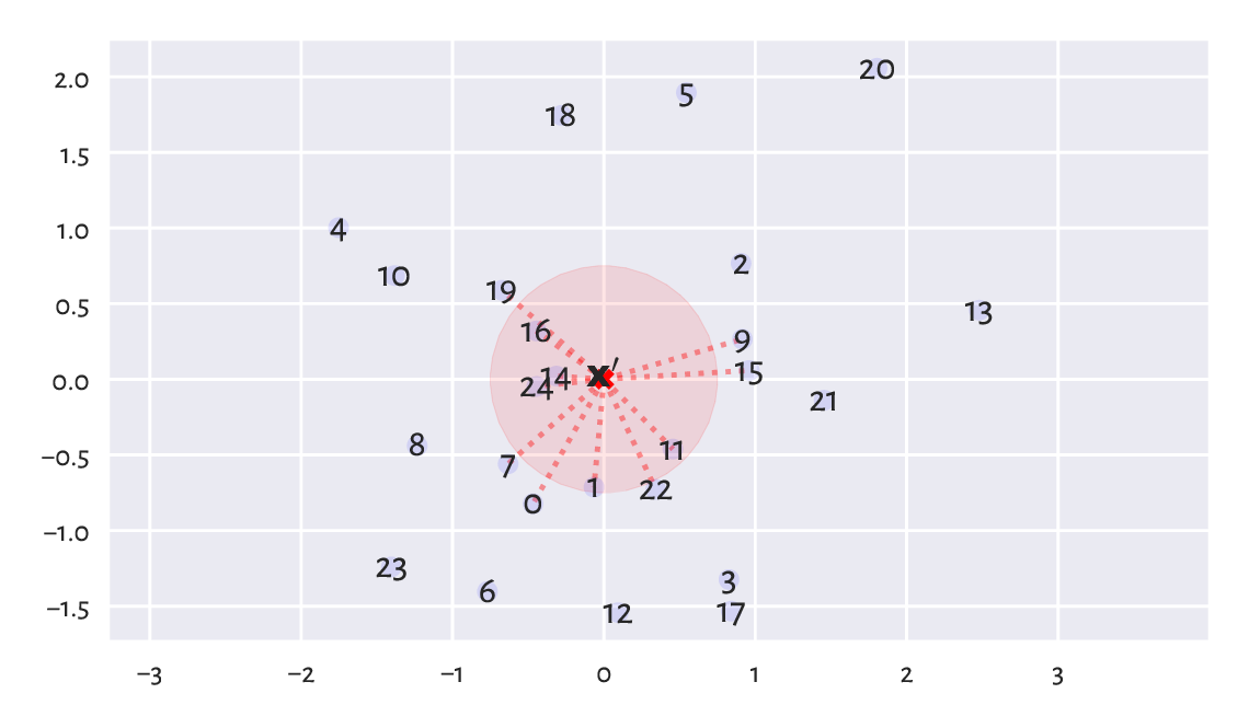
Figure 8.3 Fixed-radius search.

8.4.5. Spatial search with multidimensional binary search trees (**)

For efficiency reasons, rather than computing all pairwise distances, it is better to rely on dedicated data structures, especially if we have a large number of neighbourhood-related queries. scipy implements a spatial search algorithm based on multidimensional binary search trees called \(K\)-d trees[4].

Note

(*) In \(K\)-d trees, the data space is partitioned into hyperrectangles along the axes of the Cartesian coordinate system (standard basis). Thanks to such a representation, all subareas too far from the query point can be pruned to speed up the search.

Let’s create a data structure for searching relative to the \(\mathbf{X}\) matrix.

import scipy.spatial
T = scipy.spatial.KDTree(X)

Assume we would like to make queries with regard to three pivot points:

X_test = np.array([
    [0,  0],
    [2,  2],
    [2, -2]
])

Here are the results for the fixed radius searches \((r=0.75)\):

T.query_ball_point(X_test, 0.75)
## array([list([1, 11, 14, 16, 24]), list([20]), list([])], dtype=object)

We see that the method is nicely vectorised. We made a query about three points at the same time. As a result, we received a list-like object storing three lists representing the indexes of interest. Note that in the case of the third point, there are no elements in \(\mathbf{X}\) within the requested range (circle), hence the empty index list.

And here are the five nearest neighbours:

distances, indexes = T.query(X_test, 5)  # returns a tuple of length two

We obtained both the distances to the nearest neighbours:

distances
## array([[0.31457701, 0.44600012, 0.54848109, 0.64875661, 0.71635172],
##        [0.20356263, 1.45896222, 1.61587605, 1.64870864, 2.04640408],
##        [1.2494805 , 1.35482619, 1.93984334, 1.95938464, 2.08926502]])

and the indexes:

indexes
## array([[14, 24, 16, 11,  1],
##        [20,  5, 13,  2,  9],
##        [17,  3, 21, 12, 22]])

Each is a matrix with three rows (corresponding to the number of pivot points) and five columns (the number of neighbours sought).

Note

(*) We expect the \(K\)-d trees to be much faster than the brute-force approach (where we compute all pairwise distances) in low-dimensional spaces. Nonetheless, due to the phenomenon called the curse of dimensionality, sometimes already for \(m\ge 5\) the speed gains might be very small; see, e.g., [11].

8.5. Exercises

Exercise 8.11

Does numpy.mean(A, axis=0) compute the rowwise or columnwise means of A?

Exercise 8.12

How does shape broadcasting work? List the most common pairs of shape cases when performing arithmetic operations like addition or multiplication.

Exercise 8.13

What are the possible ways to index a matrix?

Exercise 8.14

Which kinds of matrix indexers return a view of an existing array?

Exercise 8.15

(*) How can we select a submatrix comprised of the first and the last row and the first and the last column?

Exercise 8.16

Why appropriate data preprocessing is required when computing the Euclidean distance between the points in a matrix?

Exercise 8.17

What is the relationship between the dot product, the Euclidean norm, and the Euclidean distance?

Exercise 8.18

What is a centroid? How is it defined by means of the Euclidean distance between the points in a dataset?

Exercise 8.19

What is the difference between the fixed-radius and the few nearest neighbour search?

Exercise 8.20

(*) When \(K\)-d trees or other spatial search data structures might be better than a brute-force search based on scipy.spatial.distance.cdist?

Exercise 8.21

(**) See what kind of vector and matrix processing capabilities are available in the following packages: TensorFlow, PyTorch, Theano, and tinygrad. Are their APIs similar to that of numpy?

---

[1]

This is not the same as matrix-multiply by itself which we cover in Section 8.3.

[2]

numpy.mean is amongst the many exceptions to this rule.

[3]

There are many possible distances, allowing to measure the similarity of points not only in \(\mathbb{R}^m\), but also character strings (e.g., the Levenshtein metric), ratings (e.g., cosine dissimilarity), etc. There is even an encyclopedia of distances, [25].

[4]

In our context, we would like to refer to them as \(m\)-d trees, but we decided to stick with the traditional name.